Normal Modes of Polyatomics

A normal mode of molecular vibration is a collective infinitesimal displacement pattern in which every nucleus oscillates at one angular frequency and with a fixed relative phase and amplitude. Near a stable equilibrium, mass weighting and diagonalization turn the coupled Cartesian nuclear motion into independent harmonic coordinates. Those coordinates connect four kinds of information:

• the curvature of a molecular potential-energy surface;
• the masses and equilibrium geometry of a chosen isotopologue;
• the symmetry and spatial pattern of each vibration;
• the frequencies and leading intensities expected in infrared and Raman spectra.

Normal modes are local and harmonic objects. They are not literal bond vibrations, unique atomic trajectories, or exact molecular eigenmotions at arbitrary amplitude. Their power comes from being the controlled leading approximation near an equilibrium geometry and a useful basis for systematic improvements.

Canonical Scope

This page is the canonical home for:

• the Cartesian Hessian generalized eigenproblem for a polyatomic molecule;
• mass-weighted displacements, normal coordinates, and normalization conventions;
• translation and rotation removal, including the difference between linear and nonlinear molecules;
• symmetry classification, degeneracy, and symmetry-adapted coordinates;
• first-order infrared and Raman activity of polyatomic normal modes;
• the Wilson GF internal-coordinate formulation;
• practical normal-mode calculations, validation, isotope effects, frequency scaling, and failure modes.

Coupled Oscillators: First Encounter owns the generic coupled-oscillator derivation. Oscillator as a Universal Local Model owns the general Taylor-expansion argument near a stable minimum. Potential Energy Surfaces owns stationary-point geometry and global surface construction. Here those ideas are specialized to molecular nuclear coordinates, rigid motions, spectroscopic symmetry, and computational frequency analysis. Vibrational Spectra Computation supplies an executable calibrated CO$_2$ Hessian and an anharmonic H$^{35}$Cl DVR benchmark.

Small Oscillations Around Equilibrium

Geometry and displacement vector

Consider an isolated molecule with $N$ nuclei and an equilibrium geometry

$$\mathbf R^e = \left( \mathbf R_1^e,\ldots,\mathbf R_N^e \right).$$

Collect the Cartesian displacements into a $3N$-component column vector

$$\mathbf s = \mathbf R-\mathbf R^e,$$

whose component $s_{A\alpha}$ is the displacement of nucleus $A$ along laboratory direction $\alpha\in\{x,y,z\}$. The Cartesian mass matrix is diagonal:

$$M_{A\alpha,B\beta} = M_A\delta_{AB}\delta_{\alpha\beta}.$$

Thus the mass of each nucleus is repeated for its three Cartesian components.

After the electronic problem and any declared adiabatic corrections have supplied a nuclear potential $U(\mathbf R)$, expand about the equilibrium geometry:

$$\begin{aligned} U(\mathbf R^e+\mathbf s) ={}& U_e + \left. \nabla U \right|_e^{\mathsf T}\mathbf s \\ &+ \frac12 \mathbf s^{\mathsf T} \mathbf H \mathbf s + O(s^3). \end{aligned}$$

At an unconstrained stationary geometry,

$$\left.\nabla U\right|_e=0,$$

and the Cartesian Hessian has components

$$H_{A\alpha,B\beta} = \left. \frac{\partial^2U} {\partial R_{A\alpha}\partial R_{B\beta}} \right|_e.$$

The harmonic kinetic and potential energies are therefore

$$T^{(2)} = \frac12 \dot{\mathbf s}^{\mathsf T} \mathbf M \dot{\mathbf s}, \qquad V^{(2)} = \frac12 \mathbf s^{\mathsf T} \mathbf H \mathbf s.$$

The Hessian describes curvature, but curvature alone does not determine a frequency. Nuclear masses enter through the kinetic energy.

The generalized eigenproblem

The linearized equations of motion are

$$\mathbf M\ddot{\mathbf s} + \mathbf H\mathbf s =0.$$

For a trial motion

$$\mathbf s(t) = \mathbf l_k q_k(t), \qquad q_k(t)\propto e^{-i\Omega_k t},$$

one obtains

$$\mathbf H\mathbf l_k = \Omega_k^2 \mathbf M\mathbf l_k.$$

This is a symmetric generalized eigenvalue problem. The eigenvalue is the squared angular frequency, not the frequency itself:

$$\lambda_k=\Omega_k^2.$$

For distinct eigenvalues, the displacement vectors can be chosen mass-orthonormal:

$$\mathbf l_j^{\mathsf T} \mathbf M \mathbf l_k = \delta_{jk}.$$

This metric matters. Cartesian eigenvectors that are orthogonal under the ordinary Euclidean dot product do not generally diagonalize the kinetic energy.

Mass Weighting and Normal Coordinates

Converting to an ordinary symmetric problem

Define the mass-weighted displacement

$$\mathbf x = \mathbf M^{1/2}\mathbf s$$

and the mass-weighted Hessian

$$\mathbf F = \mathbf M^{-1/2} \mathbf H \mathbf M^{-1/2}.$$

Then

$$\mathbf F\mathbf e_k = \Omega_k^2\mathbf e_k, \qquad \mathbf e_j^{\mathsf T}\mathbf e_k = \delta_{jk}.$$

The Cartesian and mass-weighted eigenvectors are related by

$$\mathbf l_k = \mathbf M^{-1/2}\mathbf e_k.$$

If the columns of $\mathbf E$ are the orthonormal vibrational eigenvectors, define normal coordinates by

$$\mathbf Q = \mathbf E^{\mathsf T}\mathbf x.$$

Equivalently,

$$Q_k = \mathbf e_k^{\mathsf T}\mathbf x = \mathbf l_k^{\mathsf T} \mathbf M\mathbf s.$$

The inverse transformation on the vibrational subspace is

$$\mathbf s = \sum_k \mathbf l_kQ_k.$$

The harmonic energies become diagonal:

$$\begin{aligned} T^{(2)} &= \frac12\sum_k\dot Q_k^2, \\ V^{(2)} &= \frac12\sum_k\Omega_k^2Q_k^2. \end{aligned}$$

Each mass-normalized $Q_k$ has dimensions of mass$^{1/2}$ times length. Some spectroscopy and quantum-chemistry programs rescale $Q_k$ or the eigenvectors, so reported displacement columns from two programs need not agree numerically even when they represent the same physical subspace.

Frequency conventions

Three related quantities are common:

$$\nu_k = \frac{\Omega_k}{2\pi}, \qquad \widetilde\nu_k = \frac{\nu_k}{c} = \frac{\Omega_k}{2\pi c}.$$

Here $\Omega_k$ is an angular frequency, $\nu_k$ is a frequency in cycles per unit time, and $\widetilde\nu_k$ is a spectroscopic wavenumber, usually reported in $\mathrm{cm}^{-1}$. A table headed “frequency” may actually contain wavenumbers. Units and the $2\pi$ convention must be checked before comparing calculations.

Removing Translation and Rotation

The $3N$ Cartesian coordinates include motion of the molecule as a whole. Internal vibration remains only after rigid translations and rotations are separated.

Translational vectors

In mass-weighted coordinates, an unnormalized translation along laboratory direction $a$ has components

$$t^{(a)}_{A\alpha} = \sqrt{M_A}\, \delta_{\alpha a}.$$

There are always three independent translations for an isolated molecule.

Rotational vectors

Place the origin at the center of mass. An infinitesimal rotation about unit vector $\widehat{\mathbf a}$ gives the mass-weighted displacement

$$\mathbf r_A^{(a)} = \sqrt{M_A}\, \widehat{\mathbf a} \times \mathbf R_A^e.$$

For a nonlinear molecule, three independent rotation vectors exist. For a linear molecule, rotation about the molecular axis moves no nucleus, so only two independent rotational displacement vectors exist.

After orthonormalizing the external vectors into the columns of $\mathbf E_{\mathrm{ext}}$, define

$$\mathbf P_{\mathrm{vib}} = \mathbf I - \mathbf E_{\mathrm{ext}} \mathbf E_{\mathrm{ext}}^{\mathsf T}.$$

The vibrational problem may be solved with the projected matrix

$$\mathbf F_{\mathrm{vib}} = \mathbf P_{\mathrm{vib}} \mathbf F \mathbf P_{\mathrm{vib}}$$

restricted to the range of $\mathbf P_{\mathrm{vib}}$. Solving in that restricted space avoids mistaking the explicit zero eigenvalues of the projected full matrix for internal vibrations.

Mode count

For $N\ge2$, the count is:

• Nonlinear molecule: $3$ translations, $3$ rotations, and $3N-6$ vibrations.
• Linear molecule: $3$ translations, $2$ rotations, and $3N-5$ vibrations.

The linear formula differs by one because rotation around the molecular axis has no infinitesimal Cartesian displacement. A monatomic species has no internal vibration and should not be forced into either formula.

Why computed external frequencies are rarely exactly zero

Exact translational and rotational invariance at an exact stationary point gives zero external eigenvalues. A calculation may instead produce small positive or negative values because of:

• incomplete geometry optimization;
• finite-difference noise or an asymmetric numerical Hessian;
• finite integration grids and thresholds;
• an external field, embedding environment, or coordinate constraint;
• imperfect projection of rigid motions;
• a geometry represented with rounded coordinates.

A low frequency is not “automatically a rotation.” Inspect the displacement vector and state the projection procedure and numerical thresholds.

What a Normal Mode Means

A collective pattern, not one bond

In mode $k$, nucleus $A$ has Cartesian displacement

$$\delta\mathbf R_A = \mathbf l_{Ak}Q_k.$$

Even a mode described informally as a C–H stretch can contain motion of many atoms. Local labels such as stretch, bend, rock, wag, or torsion are interpretations of a collective eigenvector, not definitions of the coordinate.

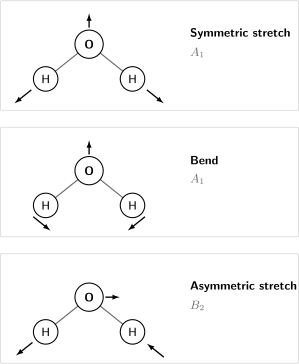
The three vibrational coordinates of nonlinear $\mathrm{H_2O}$: symmetric stretch, bend, and asymmetric stretch. Arrow lengths are schematic rather than a program-specific normalization. With $z$ along the $C_2$ axis and the molecular plane chosen as $yz$, the modes transform as $A_1$, $A_1$, and $B_2$.

Normalization is conventional

If $\mathbf l_k$ is multiplied by a nonzero constant and $Q_k$ is divided by the same constant, the Cartesian displacement is unchanged. Common outputs use mass normalization, Cartesian normalization, a chosen reduced mass, or a fixed visualization amplitude. Consequently:

• arrow length in a molecular viewer is not a zero-point amplitude;
• the largest displayed arrow need not identify the atom carrying most kinetic energy;
• “reduced mass of a mode” depends on the coordinate normalization convention;
• frequencies and invariant subspaces are more portable than raw eigenvector columns.

For the mass-normalized coordinate used here, the oscillator length is

$$Q_{\mathrm{zp},k} = \sqrt{ \frac{\hbar} {2\Omega_k} }.$$

The corresponding Cartesian zero-point displacement pattern is

$$\delta\mathbf R_{A,k}^{\mathrm{zp}} = \mathbf l_{Ak}Q_{\mathrm{zp},k}.$$

Degenerate modes are subspaces

Suppose $d$ eigenvectors share one exact eigenvalue $\Omega^2$. Any orthogonal rotation inside their span,

$$\mathbf E_d' = \mathbf E_d\mathbf O, \qquad \mathbf O^{\mathsf T}\mathbf O=\mathbf I_d,$$

is an equally valid eigenbasis. Individual columns in a degenerate pair or triplet are therefore not unique. The invariant objects are:

• the common frequency;
• the $d$-dimensional eigenspace;
• its symmetry representation;
• observables formed without privileging an arbitrary basis inside that space.

Tiny numerical symmetry breaking can rotate or split a degenerate subspace. Comparing columns one by one is then unreliable; compare subspace overlaps or symmetry-adapted combinations.

Quantizing the Harmonic Modes

Promote $Q_k$ and its conjugate momentum $P_k$ to operators:

$$[Q_j,P_k] = i\hbar\delta_{jk}.$$

The harmonic vibrational Hamiltonian is

$$H_{\mathrm{vib}}^{(2)} = \sum_{k=1}^{f} \left( \frac{P_k^2}{2} + \frac12\Omega_k^2Q_k^2 \right),$$

where

$$f = \begin{cases} 3N-6, & \text{nonlinear molecule},\\ 3N-5, & \text{linear molecule}. \end{cases}$$

Its term energies are

$$E_{\mathbf v}^{(2)} = \sum_{k=1}^{f} \hbar\Omega_k \left( v_k+\frac12 \right).$$

The exact one-dimensional oscillator eigenfunctions and ladder algebra belong to Quantum Harmonic Oscillator. The molecular result here is the reduction of a coupled polyatomic problem to a product of those oscillators.

The harmonic ground-state zero-point energy is

$$E_{\mathrm{ZP}}^{(2)} = \frac12\sum_{k=1}^{f}\hbar\Omega_k.$$

This value depends on the isotopologue through the mass matrix. It also depends on the electronic-structure model through the Hessian and is not an exact dissociation or thermochemical correction.

Symmetry Classification

Vibrational representation

At a symmetry-preserving equilibrium geometry, each point-group operation acts on the $3N$ Cartesian displacements. Let this representation be $\Gamma_{3N}$. Formally,

$$\Gamma_{\mathrm{vib}} = \Gamma_{3N} - \Gamma_{\mathrm{trans}} - \Gamma_{\mathrm{rot}}.$$

The minus signs mean subtraction of representation multiplicities after decomposition into irreducible representations. They are not set subtraction.

Because the mass-weighted Hessian commutes with every symmetry operation of the equilibrium structure, its eigenspaces can be chosen to transform as irreducible representations. Symmetry therefore:

• block-diagonalizes the normal-mode problem;
• predicts exact degeneracies required by multidimensional irreducible representations;
• distinguishes modes that cannot mix while symmetry is preserved;
• supplies selection rules for infrared and Raman activity.

Molecular Symmetry develops the point-group operations, character reductions, and water example. Here the emphasis is how those labels attach to calculated molecular vibrations.

Symmetry-adapted coordinates

Instead of diagonalizing all Cartesian displacements at once, one may first construct linear combinations that transform according to a chosen irreducible representation $\Gamma$. A projection operator has the schematic form

$$\mathcal P^{(\Gamma)} = \frac{d_\Gamma}{|G|} \sum_{g\in G} \chi^{(\Gamma)}(g)^* \widehat D(g),$$

where $d_\Gamma$ is the irrep dimension, $|G|$ is the group order, $\chi^{(\Gamma)}$ is its character, and $\widehat D(g)$ acts on displacements. Applying these projectors to trial internal coordinates produces symmetry-adapted linear combinations.

Within one symmetry block, modes of the same irrep can mix. A label such as $A_1$ does not by itself identify “the symmetric stretch”; several $A_1$ modes may exist and exchange character as geometry, isotopic composition, or computational model changes.

Water and carbon dioxide

Two small molecules expose the counting and symmetry logic:

• Water: $\mathrm{H_2O}$ is nonlinear and belongs to $C_{2v}$. It has $3(3)-6=3$ vibrational coordinates with symmetry $2A_1+B_2$.
• Carbon dioxide: $\mathrm{CO_2}$ is linear and belongs to $D_{\infty h}$. It has $3(3)-5=4$ vibrational coordinates with symmetry $\Sigma_g^+ + \Pi_u + \Sigma_u^+$.

For water, the two $A_1$ modes are conventionally called the symmetric stretch and bend, while the $B_2$ mode is the asymmetric stretch when the molecular plane is $yz$. Choosing the molecular plane as $xz$ swaps the names $B_1$ and $B_2$; some evaluated tables therefore label the same asymmetric stretch $B_1$. The displacement, degeneracy, and activity do not depend on that coordinate-label choice.

For carbon dioxide, $\Pi_u$ is two-dimensional. The two perpendicular bending coordinates share one frequency in the isolated linear molecule. Thus carbon dioxide has four vibrational coordinates but only three distinct harmonic frequencies:

$$\begin{aligned} \nu_1 &: \Sigma_g^+ \quad\text{symmetric stretch}, \\ \nu_2 &: \Pi_u \quad\text{doubly degenerate bend}, \\ \nu_3 &: \Sigma_u^+ \quad\text{antisymmetric stretch}. \end{aligned}$$

Counting named motions without counting degeneracy is a common source of the incorrect statement that a linear triatomic has only three normal modes.

Infrared Activity

Dipole derivative criterion

Expand the body-fixed electric dipole component $\mu_a$ in normal coordinates:

$$\mu_a(\mathbf Q) = \mu_a^e + \sum_k \left( \frac{\partial\mu_a} {\partial Q_k} \right)_e Q_k + O(Q^2).$$

For a harmonic fundamental from the vibrational ground state,

$$\begin{aligned} \langle1_k| \mu_a |0\rangle \approx{}& \left( \frac{\partial\mu_a} {\partial Q_k} \right)_e \langle1_k|Q_k|0\rangle \\ ={}& \left( \frac{\partial\mu_a} {\partial Q_k} \right)_e \sqrt{ \frac{\hbar} {2\Omega_k} }. \end{aligned}$$

The mode is first-order infrared active if at least one component satisfies

$$\left( \frac{\partial\mu_a} {\partial Q_k} \right)_e \ne0.$$

A permanent dipole is neither necessary nor sufficient for a particular vibrational fundamental. What matters is the dipole change along that normal coordinate.

Symmetry statement

For a nondegenerate totally symmetric vibrational ground state, the derivative can be nonzero only if $Q_k$ transforms like a component of the dipole vector. In a finite point group this is commonly stated as

$$\Gamma(Q_k) \subset \Gamma(x,y,z).$$

The more general transition rule is that

$$\Gamma(\psi_f) \otimes \Gamma(\mu_a) \otimes \Gamma(\psi_i)$$

must contain the totally symmetric representation. This form remains useful for excited vibrational states, combination bands, and vibronic coupling.

Water’s $A_1$ and $B_2$ modes all transform like allowed dipole components in $C_{2v}$, so all three fundamentals are infrared active. In carbon dioxide, the $\Pi_u$ bend and $\Sigma_u^+$ antisymmetric stretch are infrared active, while the $\Sigma_g^+$ symmetric stretch is not first-order electric-dipole active.

Raman Activity

Polarizability derivative criterion

In nonresonant Raman scattering, the leading molecular response is described by the polarizability tensor:

$$\begin{aligned} \alpha_{ab}(\mathbf Q) &= \alpha_{ab}^e + \sum_k \alpha'_{ab,k}Q_k + O(Q^2), \\ \alpha'_{ab,k} &\equiv \left( \frac{\partial\alpha_{ab}} {\partial Q_k} \right)_e. \end{aligned}$$

A harmonic fundamental is Raman active in the Placzek approximation when at least one tensor derivative is nonzero:

$$\left( \frac{\partial\alpha_{ab}} {\partial Q_k} \right)_e \ne0.$$

The relevant symmetry species are those carried by the quadratic functions

$$x^2,\ y^2,\ z^2,\ xy,\ xz,\ yz.$$

Infrared and Raman intensities probe different response derivatives. A strong infrared band need not be a strong Raman band, and a symmetry-allowed band may still be weak because its property derivative is small.

Mutual exclusion in centrosymmetric molecules

For a molecule with an inversion center:

• dipole components are ungerade;
• polarizability components are gerade;
• every normal mode has either gerade or ungerade parity.

Therefore, within the electric-dipole and first-order Raman approximations, no fundamental normal mode is both infrared and Raman active:

• A gerade mode is infrared forbidden but may be Raman active.
• An ungerade mode may be infrared active but is Raman forbidden.

“Possibly” matters: parity alone does not guarantee activity, because the full irrep must match the relevant vector or quadratic-tensor species.

Carbon dioxide illustrates the rule. Its gerade symmetric stretch is Raman active, while its ungerade bend and antisymmetric stretch are infrared active. Water has no inversion center, so the mutual-exclusion argument does not apply; its fundamentals can be active in both techniques.

Weak apparent violations can arise from symmetry breaking, isotopic substitution, crystal or solvent environments, vibronic coupling, resonance effects, anharmonic combination states, or higher multipoles. The correct conclusion is then that the idealized assumptions need refinement, not that inversion parity has ceased to be meaningful.

Internal Coordinates and the Wilson GF Method

Cartesian normal modes are straightforward computationally, but bond lengths and angles are often chemically easier to interpret. Let a nonredundant vector of infinitesimal internal coordinates be

$$\mathbf S = \mathbf B\mathbf s,$$

where $\mathbf B$ is the Wilson $B$ matrix evaluated at equilibrium. Define

$$\mathbf G = \mathbf B \mathbf M^{-1} \mathbf B^{\mathsf T}.$$

With one common convention, the harmonic energies are

$$T^{(2)} = \frac12 \dot{\mathbf S}^{\mathsf T} \mathbf G^{-1} \dot{\mathbf S}, \qquad V^{(2)} = \frac12 \mathbf S^{\mathsf T} \mathbf F_S \mathbf S.$$

The secular equation is then

$$\det \left( \mathbf G\mathbf F_S - \Omega^2\mathbf I \right) =0.$$

Although $\mathbf G\mathbf F_S$ need not look symmetric, for positive-definite $\mathbf G$ it is similar to the symmetric matrix

$$\mathbf G^{1/2} \mathbf F_S \mathbf G^{1/2}.$$

The Wilson GF method separates kinetic information, carried by geometry and masses in $\mathbf G$, from force constants in $\mathbf F_S$. It is especially valuable for symmetry coordinates, isotopic comparisons, and spectroscopic force-field fitting.

Real internal-coordinate sets may be redundant. Then $\mathbf B$ has dependent rows, $\mathbf G$ is singular on the redundant directions, and one must impose constraints or work in an independent subspace. Replacing inverses with a pseudoinverse without tracking that subspace can create spurious modes.

Isotope Substitution

Within the strict Born–Oppenheimer approximation, changing isotopes leaves the electronic potential and Cartesian Hessian unchanged but changes the mass matrix. Frequencies and eigenvectors are therefore both isotopologue dependent.

For an isolated, nondegenerate mode with

$$\mathbf H\mathbf l_k = \lambda_k\mathbf M\mathbf l_k, \qquad \mathbf l_k^{\mathsf T} \mathbf M\mathbf l_k =1,$$

a small mass change at fixed Hessian gives

$$\delta\lambda_k = - \lambda_k \mathbf l_k^{\mathsf T} \delta\mathbf M \mathbf l_k.$$

Since $\lambda_k=\Omega_k^2$,

$$\frac{\delta\Omega_k}{\Omega_k} = - \frac12 \mathbf l_k^{\mathsf T} \delta\mathbf M \mathbf l_k.$$

This first-order formula shows that isotope sensitivity is weighted by participation in the mass-normalized mode. It must be replaced by degenerate perturbation theory near degeneracies, and large substitutions should be handled by rebuilding and diagonalizing the new mass-weighted Hessian.

Isotopic substitution can:

• lower frequencies without changing the force field;
• rotate and reorder modes of the same symmetry;
• lift degeneracies when the substitution lowers molecular symmetry;
• activate bands that were symmetry forbidden in the parent isotopologue;
• help identify which atoms participate in an observed vibration.

The diatomic reduced-mass limit is developed in Vibrations of Diatomics.

Computational Normal-Mode Analysis

A reproducible workflow

A defensible calculation records the complete inference chain:

1. Specify the isotopologue, charge, spin state, electronic state, environment, electronic-structure method, basis or representation, and relativistic model if relevant.
2. Optimize the geometry with declared convergence thresholds.
3. Evaluate the Cartesian Hessian at that geometry, analytically or by finite differences.
4. Symmetrize the numerical Hessian if necessary and document the procedure.
5. Build the mass-weighted Hessian using the intended isotope masses.
6. Construct and remove the translational and rotational subspace.
7. diagonalize the vibrational block and convert eigenvalues with explicit units;
8. compute dipole and polarizability derivatives when intensities are required;
9. classify modes by symmetry and inspect displacement patterns;
10. test sensitivity to geometry, numerical thresholds, method, basis, isotope masses, and environmental model.

Capitalization in a checklist is less important than preserving this provenance. A bare list of computed wavenumbers is not reproducible evidence.

Analytic and finite-difference Hessians

An analytic Hessian evaluates second derivatives directly within the chosen electronic-structure method. If only gradients are available, a central difference gives

$$H_{ij} \approx \frac{ g_i(\mathbf R+h\mathbf e_j) - g_i(\mathbf R-h\mathbf e_j) } {2h},$$

where $g_i=\partial U/\partial R_i$.

The step $h$ must balance truncation error against numerical noise. Useful checks include:

• repeat selected columns with a smaller and larger step;
• verify $H_{ij}\approx H_{ji}$ before symmetrization;
• tighten self-consistent-field, integral, grid, and embedding tolerances;
• preserve the intended molecular orientation and electronic state;
• compare analytic and finite-difference results when both are available.

Finite differences of energies are possible but generally amplify numerical noise more severely than finite differences of gradients.

Stationary-point diagnosis

For a mass-weighted Hessian eigenvalue $\lambda_k$:

• $\lambda_k=\Omega_k^2>0$ is a stable harmonic direction.
• $\lambda_k=0$ is an exact flat or rigid direction.
• $\lambda_k=-\kappa_k^2<0$ is an unstable harmonic direction.

For $\lambda_k<0$, programs often print an “imaginary frequency”

$$\Omega_k=i\kappa_k$$

or a negative signed wavenumber. At an unconstrained local minimum, all internal eigenvalues should be positive. A first-order saddle has one negative internal eigenvalue; higher-order saddles have more.

This diagnostic requires interpretation. A small negative value dominated by translation or rotation may be numerical contamination. A constrained optimization can be a minimum on the constrained manifold while remaining unstable in a released coordinate. A geometry with nonzero gradient is not classified reliably by Hessian inertia alone.

Frequency scaling and uncertainty

Computed harmonic wavenumbers differ from measured fundamentals for two separate reasons:

• the harmonic Hessian omits vibrational anharmonicity and mode coupling;
• the electronic-structure model and numerical representation approximate the true potential.

An empirical factor is sometimes applied:

$$\widetilde\nu_k^{\mathrm{pred}} = s\, \widetilde\nu_k^{\mathrm{harm}}.$$

The factor $s$ is method-, basis-, dataset-, and target-property dependent. NIST analyses emphasize that fitted scale factors have uncertainty and often justify only about two significant digits. A scaled number is not an anharmonic calculation and should not be reported without the factor’s source, calibration domain, and uncertainty.

Do not apply one global factor mechanically to:

• imaginary modes;
• nearly free internal rotations;
• floppy or large-amplitude coordinates;
• modes strongly mixed by resonance;
• calculations outside the factor’s calibration model.

Intensities and assignments

A frequency calculation may also report infrared intensities and Raman activities. These are derived from property derivatives and use program-specific unit and orientation conventions. Validation should distinguish:

• a symmetry label from a visual mode description;
• an activity from an observed integrated intensity;
• a harmonic normal frequency from an experimental band center;
• a fundamental from an overtone, combination band, hot band, or rotationally structured band;
• an isolated-molecule result from a condensed-phase or matrix-isolation measurement.

Agreement in frequency does not establish an assignment by itself. Symmetry, isotope shifts, intensity patterns, rotational structure, temperature dependence, and anharmonic resonance information provide independent tests.

Where the Harmonic Picture Breaks

Mechanical anharmonicity

Beyond quadratic order,

$$\begin{aligned} V(\mathbf Q) &= V^{(2)}+V^{(3)}+V^{(4)}+\cdots, \\ V^{(2)} &= \frac12 \sum_k\Omega_k^2Q_k^2, \\ V^{(3)} &= \frac{1}{3!} \sum_{ijk} \Phi_{ijk}Q_iQ_jQ_k, \\ V^{(4)} &= \frac{1}{4!} \sum_{ijkl} \Phi_{ijkl}Q_iQ_jQ_kQ_l. \end{aligned}$$

The cubic and quartic force constants couple harmonic modes, shift term values, permit overtones and combination bands, and generate resonances. Harmonic quantum numbers then become approximate labels rather than exact constants of motion.

Electrical anharmonicity

Nonlinear terms in the dipole and polarizability expansions can generate intensity even when the harmonic property derivative vanishes. Mechanical and electrical anharmonicity are distinct and can reinforce or cancel one another.

Large-amplitude motion

Torsions, inversions, proton transfers, pseudorotations, and dissociation coordinates may explore regions for which one rectilinear normal coordinate is poor. Typical remedies include:

• curvilinear internal coordinates;
• hindered-rotor Hamiltonians;
• multidimensional variational calculations;
• vibrational self-consistent-field and configuration-interaction methods;
• vibrational perturbation theory with explicit resonance treatment;
• path-based or reaction-coordinate models.

Low-frequency harmonic modes also give fragile entropy estimates because the harmonic density of states grows too quickly as $\Omega\to0$. Quasiharmonic clipping can stabilize bookkeeping, but a physically justified hindered-rotor or anharmonic treatment is preferable when the coordinate is genuinely rotational.

Electronic and environmental coupling

Near electronic degeneracies, conical intersections, or strong nonadiabatic regions, one scalar Hessian on one Born–Oppenheimer surface may not organize the nuclear dynamics. Solvent, crystal, cavity, field, and embedding environments can change both the force field and the meaning of rigid translation and rotation. The model must match the physical boundary conditions.

Interpreting a Frequency Output

Before accepting a normal-mode table, ask:

Question	Why it matters
Was the geometry stationary at the same model used for the Hessian?	Residual gradients contaminate rotational modes and invalidate a simple stationary-point classification.
Which isotope masses were used?	Mass weighting controls both frequencies and mode mixing.
Were rigid motions projected?	Near-zero external motion can mix with low internal modes.
Is the reported quantity $\Omega$, $\nu$, or $\widetilde\nu$?	Factors of $2\pi$ and $c$ otherwise produce unit errors.
How are eigenvectors normalized?	Raw arrows and reduced masses are convention dependent.
Does a degeneracy follow the molecular symmetry?	Artificial splitting can expose geometry or numerical symmetry breaking.
Are intensities harmonic derivatives or simulated band strengths?	These are different observables.
Was a scale factor applied?	The factor has a calibration domain and uncertainty.
Is a low mode a vibration, hindered rotation, or environmental motion?	The harmonic thermodynamic interpretation may fail.
Were assignments tested against isotope and symmetry information?	Frequency agreement alone is underdetermined.

Common Mistakes

“There are 3N vibrational modes”

The Cartesian Hessian has dimension $3N$, but isolated molecular vibration excludes three translations and either two or three rotations.

“Every eigenvector is uniquely defined”

Its sign is arbitrary, its scale depends on convention, and a degenerate eigenspace admits arbitrary orthogonal rotations.

“A negative printed frequency is a negative energy”

The negative sign usually encodes a negative squared frequency, meaning local curvature is unstable. It is not a vibrational energy below zero.

“A normal mode is one bond moving”

Normal modes are collective. A local bond coordinate is generally a linear combination of several normal coordinates, and one normal coordinate can involve many internal coordinates.

“IR active means the molecule has a permanent dipole”

First-order vibrational activity requires a dipole derivative along the mode. The equilibrium dipole and transition dipole are different quantities.

“Centrosymmetric molecules have no active vibrations”

They obey mutual exclusion at leading order: ungerade modes may be infrared active and gerade modes may be Raman active. Some modes can still be silent.

“Scaling makes harmonic frequencies experimental”

A scale factor is an empirical bias correction with uncertainty. It does not generate mode-specific anharmonic shifts, resonance splittings, or environment effects.

Exercises

1. Derive the mass-weighted eigenproblem

Starting from

$$\mathbf H\mathbf l = \Omega^2\mathbf M\mathbf l,$$

show that $\mathbf e=\mathbf M^{1/2}\mathbf l$ satisfies an ordinary symmetric eigenproblem. Then prove the equivalence of Euclidean orthonormality of $\mathbf e_k$ and mass orthonormality of $\mathbf l_k$.

Solution

Multiply the generalized equation on the left by $\mathbf M^{-1/2}$ and insert

$$\mathbf l = \mathbf M^{-1/2}\mathbf e.$$

Then

$$\begin{aligned} \mathbf M^{-1/2} \mathbf H \mathbf M^{-1/2}\mathbf e &= \Omega^2 \mathbf M^{-1/2} \mathbf M \mathbf M^{-1/2}\mathbf e \\ &= \Omega^2\mathbf e. \end{aligned}$$

Thus

$$\mathbf F\mathbf e = \Omega^2\mathbf e, \qquad \mathbf F = \mathbf M^{-1/2} \mathbf H \mathbf M^{-1/2}.$$

Because $\mathbf H$ and $\mathbf M^{-1/2}$ are symmetric, $\mathbf F$ is symmetric. Finally,

$$\begin{aligned} \mathbf l_j^{\mathsf T} \mathbf M \mathbf l_k &= \mathbf e_j^{\mathsf T} \mathbf M^{-1/2} \mathbf M \mathbf M^{-1/2} \mathbf e_k \\ &= \mathbf e_j^{\mathsf T}\mathbf e_k = \delta_{jk}. \end{aligned}$$

2. Count modes carefully

Find the number of vibrational coordinates for:

1. nonlinear ammonia, $\mathrm{NH_3}$;
2. linear acetylene, $\mathrm{C_2H_2}$;
3. nonlinear methane, $\mathrm{CH_4}$;
4. a single argon atom.

Explain why the monatomic case is not obtained by blindly substituting $N=1$ into $3N-5$.

Solution

Ammonia has $N=4$ and is nonlinear:

$$f=3(4)-6=6.$$

Acetylene has $N=4$ and is linear:

$$f=3(4)-5=7.$$

Methane has $N=5$ and is nonlinear:

$$f=3(5)-6=9.$$

A single atom has no internal coordinate and therefore no molecular vibration. The linear-molecule count assumes at least two distinct nuclear positions defining an axis and two nontrivial rotations perpendicular to it. Those assumptions fail for $N=1$.

3. Build the vibrational projector

Let $\mathbf E_{\mathrm{ext}}$ contain orthonormal mass-weighted translation and rotation vectors. Show that

$$\mathbf P = \mathbf I - \mathbf E_{\mathrm{ext}} \mathbf E_{\mathrm{ext}}^{\mathsf T}$$

is a symmetric projector and annihilates every external vector.

Solution

Orthonormality gives

$$\mathbf E_{\mathrm{ext}}^{\mathsf T} \mathbf E_{\mathrm{ext}} = \mathbf I.$$

The matrix is symmetric because

$$\mathbf P^{\mathsf T} = \mathbf P.$$

Its square is

$$\begin{aligned} \mathbf P^2 &= \left( \mathbf I-\mathbf E_{\mathrm{ext}} \mathbf E_{\mathrm{ext}}^{\mathsf T} \right)^2 \\ &= \mathbf I - \mathbf E_{\mathrm{ext}} \mathbf E_{\mathrm{ext}}^{\mathsf T} = \mathbf P. \end{aligned}$$

Finally,

$$\mathbf P\mathbf E_{\mathrm{ext}} = \mathbf E_{\mathrm{ext}} - \mathbf E_{\mathrm{ext}} \left( \mathbf E_{\mathrm{ext}}^{\mathsf T} \mathbf E_{\mathrm{ext}} \right) =0.$$

Thus $\mathbf P$ projects orthogonally onto the complement of the rigid-motion subspace.

4. Water activity

The water vibrational representation is

$$\Gamma_{\mathrm{vib}} = 2A_1+B_2.$$

Choose $z$ along the $C_2$ axis and the molecular plane as $yz$, so $z$ transforms as $A_1$, $y$ as $B_2$, and the quadratic functions include both $A_1$ and $B_2$ species. Determine the first-order infrared and Raman activity of all three modes.

Solution

An infrared-active mode must transform like a dipole component. Both $A_1$ and $B_2$ occur among the vector components, so the two $A_1$ modes and the $B_2$ mode are infrared active.

A Raman-active mode must transform like a quadratic component of the polarizability tensor. Both species also occur among the quadratic functions, so all three are Raman active.

This does not violate mutual exclusion because $C_{2v}$ has no inversion center.

5. Carbon dioxide and degeneracy

Carbon dioxide has vibrational symmetry

$$\Sigma_g^+ + \Pi_u + \Sigma_u^+.$$

Explain why this gives four normal coordinates but three distinct harmonic frequencies. Classify the leading infrared and Raman activity.

Solution

$\Sigma_g^+$ and $\Sigma_u^+$ are one-dimensional, while $\Pi_u$ is two-dimensional. Hence

$$1+2+1=4$$

normal coordinates occur, but the two $\Pi_u$ bending coordinates are symmetry-degenerate and share one harmonic frequency.

Carbon dioxide is centrosymmetric. The ungerade $\Pi_u$ bend and $\Sigma_u^+$ antisymmetric stretch can be infrared active. The gerade $\Sigma_g^+$ symmetric stretch is Raman active. At leading order no one mode is active in both.

6. First-order isotope shift

For a nondegenerate mass-normalized mode, suppose only nucleus $A$ changes mass by $\delta M_A>0$. Use

$$\frac{\delta\Omega_k}{\Omega_k} = - \frac12 \mathbf l_k^{\mathsf T} \delta\mathbf M \mathbf l_k$$

to show that the frequency decreases and identify when the shift is small.

Solution

The mass perturbation contributes in the three Cartesian components of nucleus $A$:

$$\mathbf l_k^{\mathsf T} \delta\mathbf M \mathbf l_k = \delta M_A \sum_{\alpha=x,y,z} l_{A\alpha,k}^2.$$

Every term is nonnegative, so

$$\delta\Omega_k\le0.$$

The first-order shift is small when nucleus $A$ has little displacement in that mass-normalized mode. Near a degeneracy, however, isotope substitution can rotate the whole degenerate subspace, so nondegenerate first-order reasoning is insufficient.

7. Diagnose a computed imaginary mode

A calculation on a nominal minimum reports one internal value of $-18\,\mathrm{cm}^{-1}$. List a sequence of checks that distinguishes a true instability from numerical or rigid-motion contamination.

Solution

A useful sequence is:

1. visualize the eigenvector and measure its overlap with translations and rotations;
2. inspect the residual gradient and repeat the geometry optimization with tighter thresholds;
3. verify that the Hessian and optimization use the same electronic state, method, basis, grid, and environment;
4. tighten electronic and numerical convergence settings;
5. if finite differences were used, vary the displacement step and check Hessian symmetry;
6. reproject rigid motions using unrounded coordinates and the intended isotope masses;
7. displace the geometry in both directions along the internal component and reoptimize or map the energy.

A persistent energy-lowering internal displacement supports a real instability. A value that vanishes under better optimization, projection, or numerical convergence was not a physical imaginary vibration.

8. Basis freedom in a degenerate bend

Let $\mathbf e_1$ and $\mathbf e_2$ be orthonormal eigenvectors of a doubly degenerate bend. Define

$$\begin{aligned} \mathbf e_1' &= \cos\theta\,\mathbf e_1 + \sin\theta\,\mathbf e_2, \\ \mathbf e_2' &= - \sin\theta\,\mathbf e_1 + \cos\theta\,\mathbf e_2. \end{aligned}$$

Show that the primed vectors are also orthonormal eigenvectors and explain what should be compared between two calculations.

Solution

The transformation matrix

$$\mathbf O = \begin{pmatrix} \cos\theta & -\sin\theta\\ \sin\theta & \cos\theta \end{pmatrix}$$

is orthogonal. Therefore the primed vectors remain orthonormal. Because the Hessian acts as $\Omega^2\mathbf I$ inside the degenerate subspace,

$$\mathbf F\mathbf E_2' = \mathbf F\mathbf E_2\mathbf O = \Omega^2\mathbf E_2\mathbf O = \Omega^2\mathbf E_2'.$$

Two programs may choose different values of $\theta$, signs, or coordinate axes. Compare the common frequency, symmetry label, and projector onto the two-dimensional subspace,

$$\mathbf P_2 = \mathbf E_2\mathbf E_2^{\mathsf T},$$

rather than matching individual columns.

Key Takeaways

• Polyatomic normal modes solve a generalized Hessian eigenproblem in which the mass matrix is as essential as the force constants.
• Mass weighting converts the problem to an ordinary symmetric eigenproblem and defines coordinates with diagonal harmonic kinetic and potential energies.
• An isolated nonlinear molecule has $3N-6$ vibrational coordinates; a linear molecule has $3N-5$.
• Translation and rotation should be constructed and projected explicitly, especially when interpreting low frequencies.
• A normal mode is a collective, local displacement pattern. Its sign and scale are conventional, and a degenerate mode is fundamentally a subspace.
• Point-group symmetry classifies modes, protects degeneracies, limits mixing, and predicts first-order infrared and Raman activity.
• Infrared intensity depends on dipole derivatives; Raman activity depends on polarizability derivatives. Centrosymmetric molecules obey mutual exclusion at leading order.
• A computed frequency table is trustworthy only with geometry, isotope, method, projection, unit, normalization, and uncertainty provenance.
• Harmonic normal modes are a basis for anharmonic and large-amplitude treatments, not a claim that real molecular motion remains separable at all energies.

Cross-Links

• Common Molecular Hamiltonians places the harmonic normal-mode operator inside the wider molecular reduction hierarchy.
• Molecular Quantum Mechanics places normal modes in the electronic–vibrational–rotational hierarchy.
• Molecular Hamiltonian gives the all-particle Coulomb starting point and exact center-of-mass separation.
• Born–Oppenheimer in Molecules explains how an electronic surface becomes a nuclear Hamiltonian and where one-surface dynamics fails.
• Potential Energy Surfaces owns stationary points, Hessian geometry, reaction coordinates, and surface uncertainty.
• Vibrations of Diatomics develops the one-coordinate limit, isotope scaling, anharmonic term values, and dipole selection rules.
• Rovibrational Coupling shows how vibrational excitation changes rotational structure and how Coriolis interactions mix mode and rotational angular momenta.
• Vibrational Spectroscopy uses normal modes as spectral labels and develops anharmonic assignment, intensity, and force-field inference.
• Infrared Spectroscopy develops the dipole-coupled measurement, polarization, FTIR and ATR sampling, and fingerprint-region workflow.
• Raman Spectroscopy develops the polarizability-coupled scattering amplitude, Raman tensors, depolarization, rotational Raman structure, and resonance limit.
• Coupled Oscillators: First Encounter gives the canonical two-oscillator diagonalization and the general matrix pattern.
• Quantum Harmonic Oscillator gives exact oscillator eigenstates, ladder operators, and matrix elements.
• Oscillator as a Universal Local Model explains the quadratic approximation near a stable equilibrium.
• Selection Rules and Transition Rates separates symmetry zeros, transition operators, amplitudes, and measured rates.
• Molecular Symmetry develops point groups, vibrational representations, and molecular selection-rule machinery.
• Molecular Physics maps those tools into the wider rotation, vibration, and field-response landscape.
• Quantum Chemistry Roadmap places normal-mode analysis in a broader study sequence.
• Quantum Chemistry References provides a wider source ladder for electronic structure, nuclear motion, and spectroscopy.

References

• E. B. Wilson Jr., J. C. Decius, and P. C. Cross, Molecular Vibrations: The Theory of Infrared and Raman Vibrational Spectra, McGraw–Hill, 1955; Dover reprint, 1980.
• G. Herzberg, Molecular Spectra and Molecular Structure. II. Infrared and Raman Spectra of Polyatomic Molecules, Van Nostrand, 1945.
• P. R. Bunker and P. Jensen, Molecular Symmetry and Spectroscopy, 2nd ed., NRC Research Press, 1998.
• P. F. Bernath, Spectra of Atoms and Molecules, 5th ed., Oxford University Press, 2025, doi:10.1093/oso/9780197754498.001.0001.
• D. Papoušek and M. R. Aliev, Molecular Vibrational-Rotational Spectra, Elsevier, 1982.
• IUPAC, “normal mode”, Compendium of Chemical Terminology, 5th ed., 2025, doi:10.1351/goldbook.08648.
• IUPAC, “normal coordinate”, Compendium of Chemical Terminology, 5th ed., 2025, doi:10.1351/goldbook.08644.
• IUPAC, “normal coordinate analysis”, Compendium of Chemical Terminology, 5th ed., 2025, doi:10.1351/goldbook.08645.
• K. Nakamoto, Infrared and Raman Spectra of Inorganic and Coordination Compounds, Part A: Theory and Applications in Inorganic Chemistry, 6th ed., Wiley, 2009.
• J. M. Hollas, Modern Spectroscopy, 4th ed., Wiley, 2004.
• K. K. Irikura, R. D. Johnson III, and R. N. Kacker, “Uncertainties in Scaling Factors for Ab Initio Vibrational Frequencies,” Journal of Physical Chemistry A 109, 8430–8437 (2005), doi:10.1021/jp052793n.
• J. P. Merrick, D. Moran, and L. Radom, “An Evaluation of Harmonic Vibrational Frequency Scale Factors,” Journal of Physical Chemistry A 111, 11683–11700 (2007), doi:10.1021/jp073974n.
• NIST Computational Chemistry Comparison and Benchmark Database, Vibrational frequency scaling guidance, Standard Reference Database 101.
• NIST Chemistry WebBook, SRD 69, Water vibrational and electronic energy levels, with evaluated spectroscopic compilations.