Valence Bond Theory

Valence-bond theory represents a molecular electronic state as a linear combination of antisymmetric, spin-adapted many-electron structures built from localized one-electron orbitals. A structure may resemble a Lewis formula: electrons are assigned to localized bonds, lone pairs, radical centers, or formal-charge patterns. The quantum state is not one drawing, however. It is a variational superposition whose orbitals and coefficients can be optimized.

This definition separates quantitative valence-bond theory from three common caricatures. It is not a classical model of labeled electrons sitting on sticks, not merely a set of mnemonic hybridization rules, and not fundamentally incompatible with molecular-orbital theory. Complete VB and MO expansions span the same antisymmetric Hilbert space. They become different approximations when each retains a different compact subset of that space.

Molecular Orbitals owns LCAO mixing, orbital symmetry, occupations, and frontier-orbital language. Spin and Spatial Wavefunctions owns the general exchange-symmetry rule. This page develops the localized, spin-coupled molecular representation and its interpretation.

H₂⁺ Ion isolates the one-electron bond, for which there is no electron pair to spin-couple and no electron–electron correlation. It is therefore a useful boundary case, but not a substitute for the two-electron covalent structures developed here.

Hydrogen Molecule is the canonical worked two-electron comparison: it evaluates the normalized Heitler–London state, relates localized structures to $g^2$ and $u^2$ configurations, and follows each approximation to dissociation.

Canonical Scope

This page is the canonical home for:

• localized covalent, ionic, radical, bond, and lone-pair structures as many-electron basis functions;
• antisymmetrized products of localized orbitals and spin functions;
• spin pairing and spin-adapted VB structures;
• nonorthogonal structure overlap and the generalized secular equation;
• resonance among structures and the nonuniqueness of structure weights;
• hybridization as a localized orbital-basis choice;
• exact and approximate relations between valence-bond and molecular-orbital expansions;
• modern VBSCF, generalized-valence-bond, spin-coupled, and breathing-orbital ideas;
• validation and interpretation rules for quantitative VB calculations.

The detailed two-electron energy curve of the hydrogen molecule, including Heitler–London and molecular-orbital approximations, belongs to the dedicated canonical-system treatment. The present page uses generic two-center algebra to explain the representation without duplicating that calculation. General covalent, ionic, metallic, weak, and multicenter diagnostics belong to Chemical Bonding.

From a Lewis Structure to a Quantum State

Work at a fixed nuclear geometry $R$. Choose localized spatial orbitals

$$\varphi_1(\mathbf r;R), \ldots, \varphi_N(\mathbf r;R),$$

and a spin function of total spin $S$ and projection $M$,

$$\Theta_{SM}(\sigma_1,\ldots,\sigma_N).$$

The fermionic antisymmetrization projector is

$$\hat{\mathcal P}_{A} = \frac{1}{N!} \sum_{P\in S_N} (-1)^P\hat P.$$

A generic normalized VB structure is

$$\Phi_K = \mathcal N_K \hat{\mathcal P}_{A} \left[ \prod_{i=1}^{N} \varphi_i^{(K)}(\mathbf r_i) \, \Theta_{SM}^{(K)} \right].$$

The structure label $K$ can encode:

• which centers or fragments support the orbitals;
• which orbitals are doubly occupied, singly occupied, or empty;
• how open-shell spins are coupled;
• a formal ionic or covalent charge assignment;
• a chosen hybridization or localization pattern;
• the spatial and spin symmetry of the complete structure.

The electron indices are argument slots used before antisymmetrization. They do not label persistent particles. A statement such as “one electron on each center” means that the antisymmetric state is built from one localized orbital associated with each center, not that electron 1 remains attached to atom $A$.

Orbitals need not be orthogonal

Traditional and modern VB methods often allow localized orbitals on different centers to overlap:

$$\langle\varphi_p|\varphi_q\rangle \ne0.$$

This flexibility can make a compact localized ansatz more accurate, but it means that the resulting many-electron structures are also nonorthogonal. Their expansion coefficients cannot be read as ordinary probability amplitudes.

Some formulations impose strong orthogonality between selected orbital groups; others optimize fully nonorthogonal orbitals. “Valence-bond calculation” is therefore a family name. The orbital constraints, structure list, spin basis, and correlation treatment must be specified.

The Two-Electron Covalent Structure

Let $a(\mathbf r)$ and $b(\mathbf r)$ be normalized localized spatial orbitals, with

$$S_{ab} = \langle a|b\rangle.$$

The normalized spin singlet is

$$\chi_{00} = \frac{1}{\sqrt2} \left( \alpha(1)\beta(2) - \beta(1)\alpha(2) \right).$$

Because the spin factor is antisymmetric, the corresponding spatial factor must be symmetric. The normalized covalent singlet structure is

$$\Phi_{\mathrm{cov}}^{S=0} = \frac{ a(1)b(2)+b(1)a(2) }{ \sqrt{ 2\left(1+|S_{ab}|^2\right) } } \chi_{00}.$$

It contains one localized orbital from each center while respecting electron indistinguishability.

Triplet partner

The spin-triplet functions $\chi_{1M}$ are symmetric under spin exchange. Their spatial partner must be antisymmetric:

$$\Phi_{\mathrm{cov}}^{S=1,M} = \frac{ a(1)b(2)-b(1)a(2) }{ \sqrt{ 2\left(1-|S_{ab}|^2\right) } } \chi_{1M}.$$

This expression requires $|S_{ab}|<1$. If the two spatial orbitals become identical, the antisymmetric spatial factor vanishes, which is the Pauli exclusion principle in coordinate form.

The singlet and triplet have different spatial symmetry and therefore different kinetic, nuclear-attraction, and electron-repulsion matrix elements. Spin pairing is not an extra attractive force inserted into the Hamiltonian. It selects an allowed symmetry sector; the Hamiltonian determines the energy within that sector.

Singlet and Triplet States owns the rotational algebra, while Exchange and Correlation owns the distinction between exchange symmetry and correlation energy.

Ionic structures

Two center-localized closed-shell structures are

$$\Phi_A = a(1)a(2)\chi_{00},$$

and

$$\Phi_B = b(1)b(2)\chi_{00}.$$

Their formal charge assignments depend on the nuclear charges and inactive electrons, but their mathematical content is simple: both active electrons occupy the same localized spatial orbital.

For real $S_{ab}=S$, the structure overlaps include

$$\langle\Phi_A|\Phi_B\rangle = S^2,$$

and

$$\langle \Phi_A | \Phi_{\mathrm{cov}}^{S=0} \rangle = \frac{ \sqrt2\,S }{ \sqrt{1+S^2} }.$$

Thus “covalent” and “ionic” structures are generally not mutually exclusive outcomes of a measurement. They are overlapping variational basis functions.

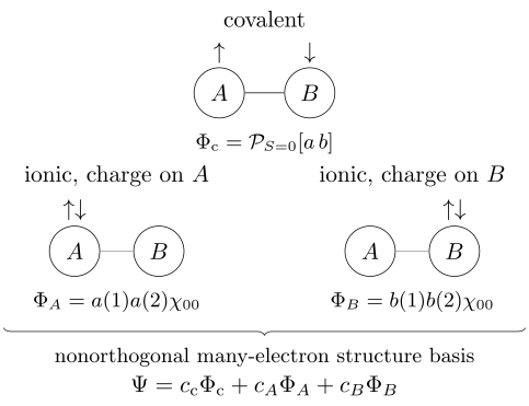
A compact two-center singlet space may contain one covalent and two ionic structures. The arrows denote localized-orbital spin occupations used to construct spin-adapted functions, not labeled electron trajectories. The physical state is the optimized superposition, and the structures may overlap.

Localized Bonds and Lone Pairs

A Lewis-like VB structure partitions the active orbital space into chemically suggestive pieces:

• two-center electron-pair bonds;
• lone pairs localized mainly on one center;
• singly occupied radical orbitals;
• empty acceptor orbitals;
• multicenter or charge-shift structures when two-center pairing is inadequate.

This partition is a representation. A localized bond orbital can be useful even when the exact density is delocalized, just as localized Wannier functions can represent a delocalized band subspace. Conversely, forcing every molecule into independent two-center pairs can hide genuine multicenter coupling, near-degeneracy, or strong resonance.

A bond structure is an ansatz

For a polar two-center singlet, a minimal VB state might be

$$|\Psi\rangle = c_{\mathrm c}|\Phi_{\mathrm{cov}}\rangle + c_A|\Phi_A\rangle + c_B|\Phi_B\rangle.$$

The ionic coefficients need not be equal in a heteronuclear molecule. Their optimized imbalance can describe polarization and charge transfer. The total electron density follows from the complete state,

$$\rho(\mathbf r) = \langle\Psi| \hat\rho(\mathbf r) |\Psi\rangle,$$

including interference between structures. It is not obtained by assigning the formal charges of the largest drawing as sharp quantum numbers.

Localized does not mean uncoupled

Each structure uses localized ingredients, but superposition can delocalize charge and spin over many centers. Matrix elements between structures communicate that coupling. A resonance expansion over local patterns is therefore entirely capable of representing global coherence.

Likewise, “a lone pair donates into an acceptor” is a controlled orbital-interaction description only after donor and acceptor subspaces are defined. In the final antisymmetric state, electrons do not retain an experimental tag recording which fragment supplied them.

Spin Pairing Beyond Two Electrons

For several open-shell orbitals, a VB structure must specify how their spins couple to total $S$. Different coupling trees span the same total-spin sector.

For $N$ spin-$1/2$ objects, the number of independent spin functions with total spin $S$ is

$$d(N,S) = \binom{N}{ \frac N2-S } - \binom{N}{ \frac N2-S-1 },$$

where a binomial coefficient outside its allowed range is zero. For four spins and $S=0$,

$$d(4,0) = \binom42-\binom41 =2.$$

There are three obvious pairwise singlet coverings, but only two are linearly independent.

Pairing diagrams can be overcomplete

Define the normalized singlet pair

$$[ij] = \frac{ \alpha(i)\beta(j) - \beta(i)\alpha(j) }{ \sqrt2 }.$$

The three four-spin pairings obey

$$[12][34] - [13][24] + [14][23] =0.$$

A set of all intuitive pairings can therefore contain exact linear dependencies. Rumer-type noncrossing diagrams provide one way to select an independent spin basis. Other coupling schemes are equally legitimate and are related by recoupling transformations.

This is why a list of bond drawings is not automatically a basis. Independence, total spin, spatial symmetry, and fermionic antisymmetry must all be checked.

Effective spin coupling

When low-energy charge fluctuations can be eliminated, two localized spin centers are often described by

$$\hat H_{\mathrm{eff}} = J\, \mathbf S_A\cdot\mathbf S_B.$$

With this convention,

$$E_{\mathrm{singlet}} = -\frac34J\hbar^2,$$

and

$$E_{\mathrm{triplet}} = \frac14J\hbar^2.$$

Thus

$$E_{\mathrm{triplet}} - E_{\mathrm{singlet}} = J\hbar^2.$$

Authors often absorb $\hbar^2$ into $J$ or use the opposite sign convention. The effective exchange parameter summarizes virtual hopping and interaction effects of an underlying electronic Hamiltonian; it is not a new fundamental force between distinguishable electrons.

Resonance as Linear Superposition

Let $\{|\Phi_K\rangle\}_{K=1}^{M}$ be linearly independent VB structures of the same exact symmetry. The variational state is

$$|\Psi\rangle = \sum_{K=1}^{M} c_K|\Phi_K\rangle.$$

Define the Hamiltonian and overlap matrices

$$H_{KL} = \langle\Phi_K|\hat H|\Phi_L\rangle,$$

and

$$S_{KL} = \langle\Phi_K|\Phi_L\rangle.$$

The Rayleigh quotient is

$$E[\mathbf c] = \frac{ \mathbf c^\dagger \mathbf H \mathbf c }{ \mathbf c^\dagger \mathbf S \mathbf c }.$$

Stationarity gives the generalized secular equation

$$\mathbf H\mathbf c = E\mathbf S\mathbf c.$$

Normalization is

$$\mathbf c^\dagger \mathbf S \mathbf c =1.$$

This is the many-electron structure-space analogue of the nonorthogonal LCAO equation. The canonical Rayleigh–Ritz derivation belongs to the Rayleigh–Ritz Method.

Linear dependence and conditioning

The overlap matrix is positive semidefinite. If

$$\mathbf S\mathbf v=0,$$

then the nominal combination

$$\sum_Kv_K|\Phi_K\rangle$$

is the zero vector. Nearly zero overlap eigenvalues indicate redundant structures and an ill-conditioned secular problem. A calculation must remove or regularize such directions before structure coefficients can be interpreted.

Symmetric two-structure example

Suppose two normalized structures have

$$H_{11}=H_{22}=h, \qquad H_{12}=H_{21}=k,$$

and

$$S_{11}=S_{22}=1, \qquad S_{12}=S_{21}=s.$$

The symmetric and antisymmetric combinations have energies

$$E_\pm = \frac{ h\pm k }{ 1\pm s }.$$

Their splitting is

$$E_--E_+ = \frac{ 2(hs-k) }{ 1-s^2 }.$$

The lower state is determined by both Hamiltonian coupling $k$ and overlap $s$. Calling $k$ alone “the resonance energy” discards the metric of the variational space.

What Resonance Structures Mean

Resonance structures are basis functions in a stationary quantum state. The molecule does not spend part of its time as one drawing and then oscillate into another. For a nondegenerate energy eigenstate,

$$|\Psi(t)\rangle = e^{-iEt/\hbar} |\Psi(0)\rangle,$$

so only the global phase changes.

Actual time-dependent transfer between localized states requires a prepared nonstationary superposition or an external perturbation. The word resonance in valence theory describes variational mixing and stabilization, not classical switching.

Resonance stabilization is reference-dependent

A positive stabilization measure can be defined as

$$\Delta E_{\mathrm{res}} = E_{\mathrm{ref}}^{\mathrm{constrained}} - E_{\mathrm{multi}}^{\mathrm{matched}}.$$

To make this meaningful, both energies must use the same Hamiltonian, one-particle basis, geometry, inactive space, correlation treatment, and orbital-optimization convention. If the multistructure calculation is allowed extra orbital relaxation or dynamic correlation, the difference contains more than structure mixing.

There is no universal Hermitian “resonance energy operator.” Different constrained references answer different chemical questions.

Why Structure Coefficients Are Not Probabilities

If the structures were orthonormal, a normalized expansion would give

$$\sum_K|c_K|^2=1,$$

and $|c_K|^2$ could be read as basis probabilities. In a nonorthogonal VB basis,

$$\sum_K|c_K|^2 \ne1$$

in general, and the structures do not represent mutually exclusive outcomes.

Chirgwin–Coulson weights

One common partition of the norm is

$$w_K^{\mathrm{CC}} = \operatorname{Re} \left[ c_K^* \left( \mathbf S\mathbf c \right)_K \right].$$

For a normalized real or complex state,

$$\sum_K w_K^{\mathrm{CC}} =1.$$

These weights can become negative or exceed one when overlap interference is strong. That behavior is not a probability paradox; it shows that the chosen partition is not a positive operator-valued decomposition.

Löwdin-orthogonalized weights

If $\mathbf S$ is positive definite, symmetric orthogonalization gives amplitudes

$$\mathbf d = \mathbf S^{1/2}\mathbf c,$$

and weights

$$w_K^{\mathrm L} = |d_K|^2.$$

They are nonnegative and sum to one, but they refer to orthogonalized combinations rather than the original raw structures. Other definitions, including inverse and projection-based weights, distribute overlap differently.

The scientifically safe practice is to report the weight definition and test whether qualitative conclusions survive reasonable orbital, structure, and weighting choices.

Hybridization as Basis Language

Hybrid orbitals are directional linear combinations within a chosen atom-centered subspace. If $\{\chi_\mu^A\}$ spans the retained valence space on center $A$, define

$$h_\lambda^A = \sum_{\mu\in A} U_{\mu\lambda} \chi_\mu^A.$$

For an orthonormal atomic subspace and unitary $\mathbf U$,

$$\mathbf U^\dagger\mathbf U = \mathbf I,$$

so the hybrids span exactly the same space as the original functions.

An idealized $sp^n$ hybrid can be written schematically as

$$h = \frac{ s+\sqrt n\,p_{\hat{\mathbf n}} }{ \sqrt{1+n} },$$

with $s$ character $1/(1+n)$ and $p$ character $n/(1+n)$ in that chosen orthonormal model. Real optimized hybrids need not have integer $n$, equivalent directions, or ideal angles.

What hybridization does not claim

• An isolated atom does not literally promote and hybridize orbitals in a timed preparatory sequence.
• A hybrid need not be an eigenfunction of the isolated atom or molecular Fock operator.
• The label $sp^2$ or $sp^3$ is not a directly measured quantum number.
• A geometry does not prove a unique hybridization; different localized bases can span the same occupied or active subspace.
• Including $d$-like polarization in a basis does not by itself establish a chemically occupied $d$ hybrid.

Atomic Orbitals Revisited owns the explicit basis-rotation interpretation of hybrids. In quantitative VB work, localized orbitals may instead be optimized directly, making a fixed textbook hybrid label optional.

The MO–VB Translation

Molecular-orbital and valence-bond theories organize the same many-electron Hilbert space differently.

Feature	Molecular-orbital organization	Valence-bond organization
one-particle functions	often orthogonal, delocalized, and symmetry-adapted	often localized and mutually nonorthogonal
many-electron basis	determinants or configuration state functions from orbital occupations	spin-coupled covalent and ionic structures
compact strength	delocalized one-electron motion and symmetry	local pairing, formal charge, and bond rearrangement
common truncation risk	too much fixed ionic character or single-reference bias	omitted structures, overlocalization, or incomplete dynamic correlation
complete-space limit	exact within the chosen one-particle basis	the same exact space when all independent structures are retained

Minimal two-center identity

Take orthonormal localized orbitals $a$ and $b$ for transparency and define

$$g = \frac{a+b}{\sqrt2}, \qquad u = \frac{a-b}{\sqrt2}.$$

The normalized closed-shell configurations are

$$\Phi_g = g(1)g(2)\chi_{00},$$

and

$$\Phi_u = u(1)u(2)\chi_{00}.$$

Define normalized symmetric covalent and ionic combinations,

$$\Phi_{\mathrm c} = \frac{ a(1)b(2)+b(1)a(2) }{ \sqrt2 } \chi_{00},$$

and

$$\Phi_{\mathrm i} = \frac{ a(1)a(2)+b(1)b(2) }{ \sqrt2 } \chi_{00}.$$

Direct expansion gives

$$\Phi_g = \frac{ \Phi_{\mathrm c} + \Phi_{\mathrm i} }{ \sqrt2 },$$

and

$$\Phi_u = \frac{ -\Phi_{\mathrm c} + \Phi_{\mathrm i} }{ \sqrt2 }.$$

Equivalently,

$$\Phi_{\mathrm c} = \frac{ \Phi_g-\Phi_u }{ \sqrt2 },$$

and

$$\Phi_{\mathrm i} = \frac{ \Phi_g+\Phi_u }{ \sqrt2 }.$$

A single closed-shell bonding-MO configuration therefore contains both covalent and ionic VB character in this minimal basis. Adding the doubly occupied antibonding configuration permits their weights to change independently. What looks like one compact structure in one representation can be a two-term expansion in another.

Equivalence and truncation

An invertible transformation of a complete one-particle basis induces an invertible transformation of the complete many-electron configuration space. Full configuration interaction in localized orbitals, canonical molecular orbitals, or any other nonsingular basis yields the same eigenvalues and physical state.

Practical methods are not complete. A one-determinant MO ansatz and a one-structure VB ansatz occupy different submanifolds. Their errors and interpretive conveniences can therefore differ greatly. “MO versus VB” is usually a comparison of truncations, orbital constraints, and optimization strategies, not of two incompatible quantum mechanics.

Dissociation and Static Correlation

A localized covalent structure naturally describes homolytic separation: each far-separated fragment retains the appropriate open-shell occupancy, while the spin coupling preserves total spin. A restricted closed-shell determinant can retain unwanted ionic terms as a bond is stretched. The Hartree–Fock Approximation gives the canonical derivation of that failure.

This does not make every truncated VB ansatz accurate at dissociation. The calculation must include:

• all fragment spin couplings needed for the target symmetry;
• ionic structures when polarization or heterolytic channels matter;
• orbital relaxation on each fragment;
• a size-consistent treatment of separated subsystems;
• dynamic correlation needed for quantitative energies;
• the correct asymptotic electronic states and nuclear charges.

Size consistency check

For noninteracting fragments at infinite separation, a size-consistent method should satisfy

$$\lim_{R\to\infty} E_{AB}(R) = E_A+E_B$$

for the specified fragment states. A compact ansatz may have the correct qualitative charge pattern yet miss this equality because its orbital restrictions or structure set do not factor into the separately optimized fragment spaces.

Static correlation describes the need for several comparably important structures or configurations. Dynamic correlation describes shorter-range avoidance around a dominant reference. The distinction is useful but not a unique observable decomposition.

Modern Quantitative VB Methods

Modern valence-bond calculations optimize wavefunctions and produce the same kinds of observables as other electronic-structure methods. Several related ansätze are common.

Method family	Variational freedom and main caution
Heitler–London type	Uses one or a few localized spin-coupled covalent structures; compact, but usually insufficient for polarization and dynamic correlation.
generalized VB	Optimizes orbital pairs and spin coupling; restrictions such as perfect pairing or strong orthogonality must be stated.
spin-coupled VB	Optimizes nonorthogonal orbitals and a flexible spin function; structure and spin-basis interpretations can be nonunique.
VBSCF	Optimizes structure coefficients and localized orbitals together; the nonlinear problem can have redundant directions and local stationary points.
VB-CI	Adds excitations or structures to a VB reference; cost grows and compact chemical interpretation can weaken.
breathing-orbital VB	Allows structure-dependent orbital relaxation; distinct orbital sets complicate overlaps and weight comparisons.
orthogonal or CASVB analysis	Transforms a multiconfigurational state into a localized VB representation; it is often an analysis of a parent state rather than an independently optimized theory.

Orbital optimization

If the orbitals depend on nonlinear parameters $\boldsymbol\kappa$, then

$$E = E( \mathbf c, \boldsymbol\kappa ).$$

VBSCF stationarity requires

$$\frac{\partial E}{\partial c_K^*}=0,$$

and

$$\frac{\partial E}{\partial\kappa_a}=0$$

subject to normalization, localization, symmetry, and any orbital constraints. Solving only the coefficient eigenproblem does not optimize the orbitals.

Because nonorthogonal orbitals and structures create gauge-like redundancies, robust implementations monitor gradient norms, overlap ranks, Hessian conditioning, multiple starting points, and invariance under allowed reparameterizations.

Dynamic correlation

A small set of chemically chosen structures often captures static correlation efficiently but misses the electron–electron cusp and short-range correlation hole. VB-CI, perturbative corrections, breathing orbitals, explicit-correlation factors, or quantum Monte Carlo can add that physics. A chemically transparent wavefunction is not automatically a quantitatively converged one.

Observables and Interpretation

A VB calculation predicts observables from the complete normalized state:

$$\langle\hat O\rangle = \mathbf c^\dagger \mathbf O \mathbf c,$$

where

$$O_{KL} = \langle\Phi_K|\hat O|\Phi_L\rangle$$

and $\mathbf c^\dagger\mathbf S\mathbf c=1$.

The off-diagonal terms matter. Replacing the expectation value by a classical average of formal structures generally discards interference.

What can be compared with experiment

• total and relative energies;
• equilibrium geometries and force constants;
• dissociation energies and asymptotes;
• dipole and higher multipole moments;
• electron and spin densities;
• transition moments and spectra;
• response properties and reaction barriers.

Structure weights, hybridization indices, resonance energies, and localized bond assignments are analysis quantities. They can be reproducible and useful, but their definitions and sensitivity must be reported.

Validation checklist

1. State the electronic Hamiltonian, geometry, charge, multiplicity, and relativistic treatment.
2. Identify active, inactive, and virtual orbital spaces.
3. State whether orbitals are orthogonal, nonorthogonal, strictly localized, or block-localized.
4. List the retained covalent, ionic, radical, and excited structures.
5. Specify the spin-coupling basis and verify $\langle S^2\rangle$.
6. Report the overlap-matrix rank and smallest retained eigenvalue.
7. State which coefficients and orbital parameters were optimized.
8. Define every quoted structure weight or resonance energy.
9. Test basis, structure-space, orbital, and correlation convergence.
10. Check dissociation, symmetry, density, and independent observable benchmarks.

Common Mistakes

• Treating one Lewis drawing as the quantum state. A quantitative VB state is usually a superposition of spin-adapted structures.
• Assigning persistent identities to electrons. Antisymmetrization removes such labels.
• Calling opposite spins distinguishable particles. Spin orbitals differ, but the electrons remain identical fermions.
• Saying spin pairing itself is an attractive force. Pairing selects symmetry; the Hamiltonian supplies the energetics.
• Interpreting resonance as rapid switching among structures. It is stationary linear superposition unless dynamics is explicitly prepared.
• Squaring coefficients in a nonorthogonal basis. Structure overlaps invalidate that probability interpretation.
• Quoting a structure weight without its definition. Chirgwin–Coulson, Löwdin, inverse, and projection weights need not agree.
• Treating hybridization as a literal atomic event. Hybrids are basis functions adapted to a representation.
• Assuming a localized orbital is unique. Orbital optimization and localization criteria can produce alternatives.
• Calling VB intrinsically more correlated than MO theory. Correlation depends on the retained many-electron space, not the vocabulary.
• Calling MO and VB fundamentally contradictory. Complete expansions are changes of representation.
• Assuming correct qualitative dissociation guarantees quantitative energy. Fragment relaxation, size consistency, and dynamic correlation still matter.
• Ignoring linear dependence. Overcomplete spin pairings or strongly overlapping structures can make the secular problem singular.
• Using formal charges as measured subsystem charges. A charge partition requires an explicit operator or real-space convention.

References

1. G. N. Lewis, “The Atom and the Molecule,” Journal of the American Chemical Society 38, 762–785 (1916), doi:10.1021/ja02261a002.
2. W. Heitler and F. London, “Wechselwirkung neutraler Atome und homöopolare Bindung nach der Quantenmechanik,” Zeitschrift für Physik 44, 455–472 (1927), doi:10.1007/BF01397394.
3. J. C. Slater, “Directed Valence in Polyatomic Molecules,” Physical Review 37, 481–489 (1931), doi:10.1103/PhysRev.37.481.
4. L. Pauling, “The Nature of the Chemical Bond. Application of Results Obtained from the Quantum Mechanics and from a Theory of Paramagnetic Susceptibility to the Structure of Molecules,” Journal of the American Chemical Society 53, 1367–1400 (1931), doi:10.1021/ja01355a027.
5. L. Pauling, “The Nature of the Chemical Bond. II. The One-Electron Bond and the Three-Electron Bond,” Journal of the American Chemical Society 53, 3225–3237 (1931), doi:10.1021/ja01360a004.
6. G. Rumer, “Zur Theorie der Spinvalenz,” Göttinger Nachrichten 3, 337–341 (1932).
7. C. A. Coulson and I. Fischer, “Notes on the Molecular Orbital Treatment of the Hydrogen Molecule,” Philosophical Magazine 40, 386–393 (1949), doi:10.1080/14786444908521726.
8. B. H. Chirgwin and C. A. Coulson, “The Electronic Structure of Conjugated Systems. VI,” Proceedings of the Royal Society A 201, 196–209 (1950), doi:10.1098/rspa.1950.0053.
9. W. J. Hunt, P. J. Hay, and W. A. Goddard III, “Self-Consistent Procedures for Generalized Valence Bond Wavefunctions,” Journal of Chemical Physics 57, 738–748 (1972), doi:10.1063/1.1678308.
10. W. A. Goddard III, T. H. Dunning Jr., W. J. Hunt, and P. J. Hay, “Generalized Valence Bond Description of Bonding in Low-Lying States of Molecules,” Accounts of Chemical Research 6, 368–376 (1973), doi:10.1021/ar50071a002.
11. P. C. Hiberty and C. Leforestier, “Expansion of Molecular Orbital Wave Functions into Valence Bond Wave Functions,” Journal of the American Chemical Society 100, 2012–2017 (1978), doi:10.1021/ja00475a007.
12. J. H. van Lenthe and G. G. Balint-Kurti, “The Valence-Bond SCF Method,” Chemical Physics Letters 76, 138–142 (1980).
13. J. H. van Lenthe and G. G. Balint-Kurti, “The Valence-Bond Self-Consistent Field Method: Theory and Test Calculations,” Journal of Chemical Physics 78, 5699–5713 (1983), doi:10.1063/1.445451.
14. D. L. Cooper, J. Gerratt, and M. Raimondi, “Applications of Spin-Coupled Valence Bond Theory,” Chemical Reviews 91, 929–964 (1991), doi:10.1021/cr00005a014.
15. P. C. Hiberty, S. Humbel, and P. Archirel, “Nature of the Differential Electron Correlation in Three-Electron Bond Dissociations,” Journal of Physical Chemistry 98, 11697–11704 (1994), doi:10.1021/j100096a012.
16. P. C. Hiberty and S. Shaik, “A Survey of Recent Developments in ab initio Valence Bond Theory,” Journal of Computational Chemistry 28, 137–151 (2007), doi:10.1002/jcc.20478.
17. S. Shaik and P. C. Hiberty, A Chemist’s Guide to Valence Bond Theory (Wiley, 2008), doi:10.1002/9780470192580.
18. G. A. Gallup, Valence Bond Methods: Theory and Applications (Cambridge University Press, 2002), doi:10.1017/CBO9780511524547.
19. R. McWeeny, Coulson’s Valence, 3rd ed. (Oxford University Press, 1979).
20. A. Szabo and N. S. Ostlund, Modern Quantum Chemistry: Introduction to Advanced Electronic Structure Theory (Dover, 1996).
21. T. Helgaker, P. Jørgensen, and J. Olsen, Molecular Electronic-Structure Theory (Wiley, 2000), doi:10.1002/9781119019572.

Exercises

1. Normalize the covalent singlet and triplet

Let $a$ and $b$ be normalized spatial orbitals with real overlap $S$. Show that

$$a(1)b(2)\pm b(1)a(2)$$

has squared norm $2(1\pm S^2)$, and identify which sign pairs with the spin singlet.

Solution

The norm is

$$\begin{aligned} &\langle ab\pm ba | ab\pm ba \rangle \\ &\quad = \langle ab|ab\rangle + \langle ba|ba\rangle \\ &\qquad \pm \langle ab|ba\rangle \pm \langle ba|ab\rangle \\ &\quad = 1+1\pm S^2\pm S^2 \\ &\quad = 2(1\pm S^2). \end{aligned}$$

The spin singlet is antisymmetric, so fermionic antisymmetry requires the symmetric spatial factor with the plus sign. The triplet pairs with the minus sign.

2. Calculate overlap among covalent and ionic structures

For real $S=\langle a|b\rangle$, use the normalized covalent singlet and $\Phi_A=a(1)a(2)\chi_{00}$ to derive

$$\langle\Phi_A|\Phi_{\mathrm{cov}}\rangle = \frac{\sqrt2S}{\sqrt{1+S^2}}.$$

What happens as $S\to0$?

Solution

The spin overlap is one. The spatial numerator gives

$$\begin{aligned} &\langle a(1)a(2)| \left[ a(1)b(2)+b(1)a(2) \right] \rangle \\ &\quad = \langle a|a\rangle \langle a|b\rangle + \langle a|b\rangle \langle a|a\rangle \\ &\quad =2S. \end{aligned}$$

Dividing by $\sqrt{2(1+S^2)}$ gives

$$\frac{2S}{\sqrt{2(1+S^2)}} = \frac{\sqrt2S}{\sqrt{1+S^2}}.$$

As $S\to0$, covalent and ionic structures become orthogonal in this minimal model.

3. Solve a nonorthogonal two-structure problem

Take

$$\begin{gathered} \mathbf H = \begin{pmatrix} -10 & -2\\ -2 & -10 \end{pmatrix}, \\[0.5em] \mathbf S = \begin{pmatrix} 1 & 0.20\\ 0.20 & 1 \end{pmatrix}. \end{gathered}$$

with energies in electronvolts. Find the two generalized eigenvalues and compare them with the result obtained by incorrectly setting $\mathbf S=\mathbf I$.

Solution

The symmetric and antisymmetric energies are

$$E_+ = \frac{-10-2}{1+0.20} = -10.0\ \mathrm{eV},$$

and

$$E_- = \frac{-10+2}{1-0.20} = -10.0\ \mathrm{eV}.$$

Here $k=hs$, so Hamiltonian coupling and overlap exactly cancel in the generalized splitting. If overlap is incorrectly discarded, the matrix eigenvalues would be

$$-12\ \mathrm{eV}, \qquad -8\ \mathrm{eV}.$$

The example is deliberately stark: a coupling matrix element cannot be interpreted without the metric of the nonorthogonal structure space.

4. Compare coefficient squares with norm weights

Two normalized structures have overlap $s=1/2$. Let

$$|\Psi\rangle = c \left( |\Phi_1\rangle+|\Phi_2\rangle \right).$$

Normalize the state and compute the two Chirgwin–Coulson weights.

Solution

Normalization gives

$$1 = c^2 \left( 2+2s \right),$$

so

$$c = \frac{1}{\sqrt{2(1+s)}} = \frac{1}{\sqrt3}.$$

The coefficient squares sum to

$$2c^2 = \frac23,$$

not one. For either structure,

$$\begin{aligned} w_1^{\mathrm{CC}} &= c \left( c+sc \right) \\ &= c^2(1+s) \\ &= \frac12. \end{aligned}$$

By symmetry $w_2^{\mathrm{CC}}=1/2$, and the two norm partitions sum to one.

5. Translate between MO and VB configurations

For orthonormal $a,b$, verify that

$$\Phi_{\mathrm c} = \frac{ \Phi_g-\Phi_u }{ \sqrt2 },$$

using $g=(a+b)/\sqrt2$ and $u=(a-b)/\sqrt2$. Explain the dissociation lesson without referring to electron trajectories.

Solution

Expanding the two closed-shell spatial products gives

$$\begin{aligned} g(1)g(2) ={}& \frac12 \bigl[ a(1)a(2) +a(1)b(2) \\ &+ b(1)a(2) +b(1)b(2) \bigr], \end{aligned}$$

and

$$\begin{aligned} u(1)u(2) ={}& \frac12 \bigl[ a(1)a(2) -a(1)b(2) \\ &- b(1)a(2) +b(1)b(2) \bigr]. \end{aligned}$$

Their difference removes the two ionic products and leaves the symmetric covalent product. After normalization and multiplication by $\chi_{00}$,

$$\frac{\Phi_g-\Phi_u}{\sqrt2} = \Phi_{\mathrm c}.$$

The lesson is representational: a correlated covalent state requires two closed-shell MO configurations in this minimal basis, while it is one compact VB structure. No electron is assigned a persistent path or identity.

6. Show that three singlet pairings are dependent

Expand $[12][34]$, $[13][24]$, and $[14][23]$ in the product-spin basis and verify

$$[12][34]-[13][24]+[14][23]=0.$$

Why does this matter computationally?

Solution

Each product contains four terms. Collecting coefficients of the six product states with two $\alpha$ and two $\beta$ spins shows pairwise cancellation in the stated combination. For example, the coefficient of $\alpha\beta\alpha\beta$ is

$$\frac12+0-\frac12=0,$$

and the coefficient of $\alpha\alpha\beta\beta$ is

$$0-\frac12+\frac12=0.$$

The remaining four coefficients cancel in the same way. Computationally, retaining all three pairings makes the spin overlap matrix singular. One must choose an independent spin basis or explicitly remove the null direction.

7. Prove hybrid-subspace invariance

Let atom-centered orbitals transform as

$$|h_\lambda\rangle = \sum_\mu|\chi_\mu\rangle U_{\mu\lambda},$$

with unitary $\mathbf U$. Show that the projector onto the retained atomic subspace is unchanged.

Solution

The transformed projector is

$$\begin{aligned} \sum_\lambda |h_\lambda\rangle \langle h_\lambda| &= \sum_{\lambda\mu\nu} |\chi_\mu\rangle U_{\mu\lambda} U_{\nu\lambda}^* \langle\chi_\nu| \\ &= \sum_{\mu\nu} |\chi_\mu\rangle \delta_{\mu\nu} \langle\chi_\nu| \\ &= \sum_\mu |\chi_\mu\rangle \langle\chi_\mu|. \end{aligned}$$

Hybridization changes the basis vectors, not the spanned subspace. An individual hybrid can still be useful because it aligns the representation with a bond direction.

8. Design a trustworthy resonance comparison

A calculation reports a $50\ \mathrm{kJ\,mol^{-1}}$ “resonance energy” by subtracting a separately optimized one-structure energy from a multistructure energy computed with extra breathing orbitals. Identify the ambiguity and propose a controlled comparison.

Solution

The difference mixes at least two effects:

1. linear mixing among VB structures;
2. extra structure-dependent orbital relaxation from breathing orbitals.

It may also mix different dynamic-correlation spaces if the calculations are not matched. A controlled resonance comparison holds the Hamiltonian, geometry, one-particle basis, inactive space, orbital constraints, and correlation model fixed. One then compares the multistructure energy with a clearly defined constrained reference in the same variational framework. A second calculation can separately quantify the additional lowering from orbital breathing. The reported value should name both references and its sign convention.