Nonadiabatic Coupling

Nonadiabatic coupling is the coupling between electronic channels generated by nuclear motion through a geometry-dependent electronic basis. It is not an extra force added to the molecular Hamiltonian. It appears because the nuclear kinetic-energy operator differentiates both the nuclear amplitudes and the electronic states used to expand the exact molecular wavefunction.

This mechanism explains why a molecule can change electronic character without absorbing or emitting another photon. It underlies internal conversion, predissociation, charge and energy transfer, vibronic intensity borrowing, and much of excited-state photochemistry. It also exposes a basic limitation of the one-surface picture:

$$\begin{gathered} \text{heavy nuclei} \\ \not\Rightarrow \\ \text{one electronic surface} \\ \text{is always isolated}. \end{gathered}$$

Whether a one-surface approximation works depends on the electronic gaps, the variation of electronic projectors with geometry, the nuclear momentum distribution, the region explored by the wavepacket, the elapsed time, and the observable. Born–Oppenheimer failure is therefore not a universal percentage attached to a molecule.

Canonical Scope

This page is the canonical molecular guide to:

• the physical meaning of off-diagonal derivative couplings;
• adiabatic and diabatic descriptions of the same coupled dynamics;
• electronic transitions at avoided crossings;
• nuclear wavepacket branching and electronic coherence;
• the assumptions, strengths, and failure modes of surface hopping;
• linear vibronic-coupling models and mode selection;
• nonradiative photochemical pathways;
• the distinction between population transfer and molecular Berry phase;
• validation and uncertainty for nonadiabatic simulations.

Born–Oppenheimer Approximation as Scale Separation owns the complete Born–Huang channel derivation, mass scaling, gauge covariance, and mathematical validity criteria. Born–Oppenheimer in Molecules owns the molecular approximation hierarchy, diagonal corrections, rovibrational applications, and precision correction ledger. Potential Energy Surfaces owns molecular landscape geometry and fitted representations. Conical Intersections owns degeneracy conditions, branching-space codimension, seam geometry, MECIs, and their computational diagnostics. Born–Oppenheimer Berry Phase owns the geometric connection, holonomy, and nuclear boundary condition.

Detailed electronic-structure algorithms, derivative-coupling implementations, molecular-dynamics integrators, software workflows, and production input choices belong to Computational Quantum Mechanics. Here the aim is to understand what a nonadiabatic model retains, what it discards, and how to test its physical claims.

Nuclear Kinetic Energy and Derivative Couplings

Exact channel expansion

After exact center-of-mass separation, write the internal Hamiltonian schematically as

$$H_{\mathrm{int}} = T_N+H_e(R),$$

where $R$ denotes internal nuclear coordinates. At each geometry, let

$$H_e(R)|\phi_a(R)\rangle = E_a(R)|\phi_a(R)\rangle.$$

An exact molecular state can be expanded as

$$|\Psi\rangle = \sum_a \chi_a(R)|\phi_a(R)\rangle$$

when the electronic basis is complete. For Cartesian nuclear coordinates, define

$$\begin{aligned} \mathbf d_{ab}^{A}(R) &= \langle\phi_a|\nabla_A\phi_b\rangle_e, \\ \tau_{ab}^{A}(R) &= \langle\phi_a|\nabla_A^2\phi_b\rangle_e. \end{aligned}$$

The off-diagonal kinetic coupling operator is

$$\hat C_{ab} = -\sum_A\frac{\hbar^2}{2M_A} \left( 2\mathbf d_{ab}^{A}\!\cdot\!\nabla_A +\tau_{ab}^{A} \right),$$

and the coupled nuclear equations take the compact form

$$\sum_b \left\{ \delta_{ab} \left[T_N+E_b(R)\right] +\hat C_{ab} \right\}\chi_b = E\chi_a.$$

No electronic transition has been inserted by hand. The coupling follows from using an $R$-dependent electronic basis under $T_N$.

What the first-derivative coupling means

The vector $\mathbf d_{ab}^{A}$ measures how electronic state $b$ rotates toward state $a$ when nucleus $A$ moves. It is a connection in electronic-state space, not a force and not by itself an observable. For nondegenerate exact eigenstates,

$$\mathbf d_{ab}^{A} = \frac{ \langle\phi_a| \nabla_AH_e |\phi_b\rangle_e }{E_b-E_a}, \qquad a\ne b.$$

This off-diagonal Hellmann–Feynman identity shows why small gaps are dangerous, but it also prevents an oversimplification. The numerator can vanish by symmetry, and a finite coupling matters dynamically only where the nuclear state has support and momentum.

Along a semiclassical path $R(t)$, a useful local diagnostic is

$$\eta_{ab}(t) = \frac{ \hbar \left| \dot R\!\cdot\!\mathbf d_{ab} \right| }{ |E_b-E_a| }.$$

The condition $\eta_{ab}\ll1$ supports adiabatic following in that chosen representation and region. It is not a transition probability and does not replace a wavepacket calculation.

Orthonormality constrains the connection

Differentiating $\langle\phi_a|\phi_b\rangle=\delta_{ab}$ gives

$$\mathbf d_{ab}^{A} = -\left(\mathbf d_{ba}^{A}\right)^*.$$

Thus the derivative-coupling matrix is anti-Hermitian. For a locally real normalized state, the diagonal element can often be set to zero by a local sign or phase convention. A global obstruction may remain around a degeneracy.

Mass suppression is not absolute protection

The coupled operator carries $1/M_A$, which is the origin of the heavy–light hierarchy. Yet its first-derivative term acts on a nuclear wavefunction whose local phase gradient is a momentum. Schematically,

$$\frac{\hbar^2}{M_A} \mathbf d_{ab}^{A}\!\cdot\!\nabla_A \sim \hbar \mathbf v_A\!\cdot\!\mathbf d_{ab}^{A}.$$

A small electronic gap, a rapidly varying eigenspace, a fast collision, or a highly excited nuclear packet can therefore defeat naive mass counting.

Adiabatic and Diabatic Representations

The coupling can move, but not disappear

In the adiabatic basis, the electronic potential matrix is diagonal and derivative couplings appear in the nuclear kinetic operator. Under an $R$-dependent unitary transformation $U(R)$ within a retained electronic subspace,

$$|\phi'_a\rangle = \sum_b|\phi_b\rangle U_{ba},$$

the potential and first-derivative connection transform as

$$\begin{aligned} \mathbf W' &= U^\dagger\mathbf E U, \\ \mathbf d' &= U^\dagger\mathbf d U +U^\dagger\nabla U. \end{aligned}$$

A diabatic or quasi-diabatic representation chooses smoother electronic vectors and accepts off-diagonal potential couplings in $\mathbf W'$. A consistent transformation leaves physical predictions unchanged. It does not turn a coupled problem into independent surfaces.

Strict and practical diabatization

A strictly diabatic basis would remove derivative coupling throughout a region. Such a basis need not exist globally, especially around conical intersections. Practical calculations instead construct quasi-diabatic states by following orbital character, transition properties, localized charge, overlaps, or a chosen optimization criterion.

The resulting matrix elements depend on the construction. Validation therefore compares transformed observables or total dynamics, not the visual smoothness of one diabatic curve.

Phase consistency is numerical physics

Electronic eigenvectors returned at neighboring geometries have arbitrary phases. Multiplying one real eigenvector by $-1$ changes the sign of its off-diagonal derivative couplings and overlaps. Random sign flips can create artificial spikes and destroy time propagation even though every isolated electronic calculation is correct.

State tracking must therefore use overlaps, projectors, symmetry labels, or another phase-consistent procedure. Near a genuine degeneracy, tracking a multidimensional electronic subspace is more robust than assigning a unique label to each eigenvector.

Avoided Crossings

A two-state local model

Consider a smooth diabatic Hamiltonian along one coordinate $Q$,

$$\mathbf W(Q) = \begin{pmatrix} \alpha Q & V\\ V & -\alpha Q \end{pmatrix}.$$

Its adiabatic energies are

$$E_\pm(Q) = \pm\sqrt{\alpha^2Q^2+V^2},$$

with minimum gap

$$\Delta E_{\min} = 2|V|.$$

Far to either side, each adiabatic eigenstate approaches one diabatic character. Across the avoided crossing, the lower adiabatic state changes character continuously. This yields two equivalent descriptions of a passage:

• adiabatic following: remain on one adiabatic surface while electronic character changes;
• diabatic passage: retain approximately the same electronic character while changing adiabatic surface.

Confusing these labels reverses verbal statements about whether a transition occurred.

Gap, speed, and coupling region

The derivative coupling is concentrated where the mixing angle changes most rapidly, usually near the minimum gap. A slower passage favors adiabatic following; a faster passage can preserve diabatic character. The Landau–Zener Transition gives the canonical probability for an ideal linear two-level sweep.

A molecular crossing rarely satisfies every Landau–Zener assumption. Real nuclear states have a momentum distribution, several coordinates can participate, the packet can revisit the coupling region, more than two electronic states may be nearby, and interference can connect several passages. A static minimum gap is therefore not a complete dynamical model.

Crossings protected by symmetry

Two states of different exact symmetry can cross along one coordinate without mixing. In the off-diagonal identity, symmetry can force

$$\langle\phi_a| \nabla_AH_e |\phi_b\rangle_e =0.$$

A small or vanishing gap then does not automatically imply transfer. If nuclear motion lowers the symmetry or a different vibrational mode has the required symmetry, the coupling can turn on. The full accessible nuclear space matters.

Nuclear Wavepacket Branching

Population transfer is coherent dynamics

Suppose two channels are retained:

$$\begin{aligned} |\Psi(t)\rangle ={}&\chi_1(R,t)|\phi_1(R)\rangle \\ &+\chi_2(R,t)|\phi_2(R)\rangle. \end{aligned}$$

As the packet reaches a coupling region, amplitude can flow between the two nuclear components. The outgoing pieces can occupy different regions of phase space and accumulate different phases. If they later overlap, their relative phase affects interference and observables.

This is why an electronic population history alone is incomplete. A faithful quantum description can require:

• where each nuclear branch travels;
• its momentum and spreading;
• coherence between branches;
• tunneling and zero-point constraints;
• return passages and interference;
• absorption or dissociation boundary conditions.

Channel population is representation dependent

Within a geometry-dependent electronic subspace, the quantity called “population of state $a$” changes under a unitary rotation of that basis. Adiabatic, diabatic, charge-localized, and spin-mixed populations answer different questions.

Asymptotic product probabilities, total density, emitted spectra, and other operational observables are less ambiguous. When reporting transient populations, state the electronic representation and population estimator.

Families of Nonadiabatic Dynamics

No single method is universally “beyond Born–Oppenheimer.” Methods retain different parts of the coupled quantum problem.

The exact coupled-channel equations retain quantum nuclei. Classical nuclei enter only after an additional mixed quantum–classical approximation, as in Ehrenfest dynamics or ordinary trajectory surface hopping. “Nonadiabatic” and “classical nuclei” are not synonyms.

• Grid or basis-set wavepacket propagation. Nuclei are fully quantum in selected coordinates, and the electronic model is a set of coupled surfaces or a diabatic matrix. Coherence, tunneling, branching, and interference are explicit. Dimensional cost and reduced-coordinate model error are the characteristic limitations.
• MCTDH and related tensor expansions. A variational quantum nuclear wavefunction evolves under a coupled vibronic Hamiltonian. The tensor structure can make correlated multimode dynamics efficient, but both the mode representation and potential representation must be converged.
• Gaussian wavepacket and multiple-spawning methods. Moving quantum basis functions represent nuclei while coupled electronic states are often computed on the fly. These methods retain phase information during packet bifurcation; spawning rules, basis completeness, and electronic cost require checks.
• Ehrenfest mean field. Classical trajectories move under a force averaged over coherent electronic amplitudes. The method is simple and can preserve short-time coherence, but one mean force can place the nuclei on no physical product surface.
• Trajectory surface hopping. An ensemble of classical trajectories moves on active surfaces while coherent amplitudes generate stochastic switches. It gives an affordable branching picture for many molecular degrees of freedom; decoherence, frustrated hops, detailed balance, tunneling, and interference remain approximate.
• Nonadiabatic perturbation or effective-mass methods. Quantum or semiclassical nuclear motion stays near one surface while excluded channels are treated perturbatively. This is effective for precision level shifts and weak couplings away from degeneracy, but fails when transfer or near-degeneracy is nonperturbative.

The table is a model map, not an accuracy ranking. Electronic-structure error, nuclear-dynamics approximation, initial-state sampling, and finite simulation time are separate axes.

Surface Hopping Overview

Mixed quantum–classical ansatz

Along a classical nuclear trajectory $R(t)$, expand the electronic state as

$$|\psi_e(t)\rangle = \sum_a c_a(t)|\phi_a(R(t))\rangle.$$

In an adiabatic basis, the coefficients obey

$$i\hbar\dot c_a = E_a(R)c_a -i\hbar\sum_b \dot R\!\cdot\!\mathbf d_{ab}(R)c_b.$$

Meanwhile, one active surface $s$ supplies the classical force,

$$M_A\ddot R_A = -\nabla_AE_s(R).$$

The electronic amplitudes evolve continuously. A stochastic rule switches the active surface so that an ensemble of trajectories follows the electronic population flow as closely as the chosen algorithm allows.

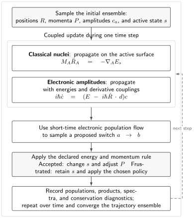
Surface hopping combines continuous electronic amplitudes with classical trajectories on active adiabatic surfaces. A proposed hop is an algorithmic branch decision, not a microscopic measurement event. Momentum adjustment, frustrated-hop handling, decoherence, and ensemble convergence are part of the physical approximation.

Fewest-switches logic

In fewest-switches surface hopping, hop probabilities are constructed from short-time changes of the electronic density matrix. The algorithm seeks the smallest number of switches consistent with the evolving electronic populations. A conceptual trajectory cycle is:

1. sample nuclear positions and momenta and choose an initial electronic preparation;
2. propagate nuclei on the active surface;
3. propagate the electronic coefficients with energies and derivative couplings;
4. use a random number to accept or reject a possible state switch;
5. adjust momentum for an accepted hop according to the energy rule;
6. repeat and form observables from a converged trajectory ensemble.

These steps leave important choices open: time step, electronic propagator, phase tracking, hop direction, decoherence correction, frustrated-hop policy, state representation, thermostat or environment model, and population estimator.

Surface hopping also carries two natural population estimates: the ensemble fraction whose active state is $a$, and the ensemble average of $|c_a|^2$. Fewest-switches logic is designed to keep them close, but they need not agree exactly in a finite or overcoherent ensemble. Persistent disagreement is a useful diagnostic rather than a quantity to hide.

Energy-conserving momentum adjustment

For an isolated spin-free trajectory, a proposed hop from $a$ to $b$ often changes momentum along a selected direction $\hat{\mathbf n}$. The scalar $\alpha$ is chosen from

$$\begin{aligned} &\frac12 \left(\mathbf P+\alpha\hat{\mathbf n}\right)^T \mathbf M^{-1} \left(\mathbf P+\alpha\hat{\mathbf n}\right) +E_b \\ &\qquad= \frac12\mathbf P^T\mathbf M^{-1}\mathbf P +E_a. \end{aligned}$$

The derivative-coupling direction is a common choice for $\hat{\mathbf n}$ in a real adiabatic two-state problem. If an upward hop has no real energy-conserving solution, it is called frustrated. Different treatments of that event can alter reflection, recrossing, and detailed balance.

Decoherence and branch separation

The electronic coefficients on one classical trajectory can remain coherent even after the corresponding nuclear branches should have separated on different surfaces. Standard fewest-switches dynamics therefore tends to overcohere in many regimes. Decoherence corrections attempt to repair this, but they are additional approximations rather than consequences of the original algorithm.

This issue is structural. One trajectory carries one nuclear position and momentum, while the exact state can contain several spatially separated packets. An ensemble creates statistical branching, but it does not automatically restore quantum phase relations between branches.

What a hop is not

A surface hop is not evidence that a molecule undergoes a literal projective measurement at one instant. It is an algorithmic device for representing coupled electronic–nuclear dynamics with classical trajectories. Individual hop times and paths are generally not observables.

Robust conclusions concern ensemble quantities that survive changes in time step, sampling, state representation, electronic method, and reasonable algorithmic variants.

Vibronic Coupling

Electronic and vibrational motion in one Hamiltonian

Vibronic coupling means coupling between electronic states and nuclear vibrational coordinates. Near a reference geometry, mass-weighted normal coordinates $Q_\kappa$ provide a useful local basis.

In mass-weighted atomic units, the reference kinetic operator is

$$T_N = -\frac12\sum_\kappa \frac{\partial^2}{\partial Q_\kappa^2}.$$

The linear vibronic-coupling Hamiltonian then has the form

$$\begin{aligned} \mathbf H_{\mathrm{LVC}} ={}& T_N\mathbf 1 +\frac12\sum_\kappa \omega_\kappa^2Q_\kappa^2\mathbf 1 \\ &+\mathbf W^{(0)} +\sum_\kappa \mathbf W_\kappa^{(1)}Q_\kappa. \end{aligned}$$

Here the matrices act in a selected diabatic electronic space. For two states, one may write

$$\mathbf W(Q) = \begin{pmatrix} W_{11}(Q) & W_{12}(Q) \\ W_{12}(Q) & W_{22}(Q) \end{pmatrix}.$$

The entries are

$$\begin{aligned} W_{11}(Q) &=E_1^0+\sum_\kappa k_{1\kappa}Q_\kappa, \\ W_{22}(Q) &=E_2^0+\sum_\kappa k_{2\kappa}Q_\kappa, \\ W_{12}(Q) &=V_{12}^0+\sum_\kappa\lambda_\kappa Q_\kappa. \end{aligned}$$

The differences $k_{1\kappa}-k_{2\kappa}$ tune the diabatic energy gap. The constant $V_{12}^0$ is the interstate coupling at the reference geometry, while $\lambda_\kappa$ measures its linear change and identifies coupling or promoting modes. Symmetry can force $V_{12}^0$ or selected $\lambda_\kappa$ to vanish.

Symmetry selects promoting modes

At a symmetry-preserving reference geometry, electronic states with irreducible representations $\Gamma_a$ and $\Gamma_b$ can couple linearly through normal mode $Q_\kappa$ only if

$$\Gamma_a \otimes \Gamma(Q_\kappa) \otimes \Gamma_b$$

contains the totally symmetric representation. Symmetry removes forbidden matrix elements; it does not determine their magnitude when they are allowed.

Local model, declared domain

An LVC model is a Taylor expansion, not a global potential-energy surface. It can fail when the dynamics reaches:

• large-amplitude torsion, dissociation, or bond rearrangement;
• strongly anharmonic coordinates;
• regions where quadratic or higher-order interstate coupling matters;
• electronic states omitted from the model;
• geometries far from the reference normal-mode frame.

Quadratic vibronic-coupling models, multiple reference geometries, on-the-fly electronic structure, or a global diabatic representation may then be needed.

Photochemistry

Photoexcitation prepares a nuclear wavepacket

In the electric-dipole approximation, an ultrashort optical preparation acts schematically as

$$|\Psi(0^+)\rangle \propto \mathbf e\!\cdot\!\boldsymbol\mu |\Psi_g\rangle.$$

The nuclei have little time to move during a sufficiently sudden excitation, but the state produced is not a point at the Franck–Condon geometry. It is a nuclear wavepacket, possibly a coherent superposition on several excited electronic surfaces, weighted by transition dipoles and the pulse spectrum.

Competing pathways

After excitation, the packet can:

• remain on an excited surface and fluoresce;
• transfer between states of the same spin multiplicity by internal conversion;
• change spin character through spin–orbit coupling and intersystem crossing;
• dissociate, isomerize, transfer charge, or reach a reactive product channel;
• lose phase and energy to an environment.

Spin-free derivative coupling does not by itself produce intersystem crossing. A model of spin-changing dynamics must include spin–orbit matrix elements and use a consistent spin-diabatic or spin-adiabatic representation.

Coupling regions as funnels, not guarantees

Conical intersections and narrow avoided crossings can provide efficient nonradiative pathways, but reaching such a region does not fix the outcome. Branching depends on the incoming nuclear position and momentum distribution, electronic coherence, topography, competing states, repeated passages, and environmental relaxation.

Likewise, a short excited-state lifetime does not by itself identify one intersection geometry. Spectroscopy and dynamics constrain pathways only through a model connecting observables to the evolving molecular state.

Quantum yield is an asymptotic question

A product quantum yield is not the population of one adiabatic state at an arbitrary simulation time. It requires product definitions, sufficiently long propagation or justified absorbing boundaries, initial-condition averaging, and treatment of all relevant competing channels. When trajectories stop early, the residual unassigned population is part of the uncertainty ledger.

Relation to Berry Phase

Diagonal and off-diagonal geometry

The same geometry dependence produces two conceptually different effects:

• off-diagonal $\mathbf d_{ab}$ transfers amplitude between electronic channels;
• diagonal $\mathbf d_{aa}$ defines a geometric connection for nuclear motion retained on one channel.

For an isolated surface, the Berry connection is

$$\boldsymbol{\mathcal A}_a(R) = i\hbar \langle\phi_a|\nabla_R\phi_a\rangle_e.$$

A closed loop $C$ can accumulate

$$\gamma_a[C] = \frac{1}{\hbar} \oint_C \boldsymbol{\mathcal A}_a\!\cdot\!dR.$$

Around a conical intersection, the one-surface electronic state can acquire a sign change, modifying nuclear interference and boundary conditions.

Choose the model by the path

A loop that remains in a gapped region can require a one-surface geometric phase even when population transfer is negligible. A packet passing through the degeneracy region generally requires several coupled electronic states. Adding a Berry sign to one scalar surface is not a substitute for dynamics through a gap-closing region.

Born–Oppenheimer Berry Phase is the canonical home for the gauge transformation, Born–Huang scalar term, holonomy, and molecular sign rule.

Accuracy, Cost, and Interpretation

Separate the error axes

For a simulated observable $O$, keep at least the following uncertainties distinct:

Axis	Typical source	Diagnostic
Hamiltonian	relativity, spin–orbit terms, environment, external field	enlarge the physical model and compare correction scales
electronic structure	wrong state ordering, poor gradients or couplings, missing correlation	benchmark energies, forces, characters, and couplings along relevant paths
electronic subspace	omitted nearby states or continua	enlarge the retained state manifold
nuclear dynamics	classical nuclei, reduced dimensions, missing tunneling or interference	compare with a quantum treatment on a reduced benchmark
initial ensemble	temperature, pulse bandwidth, Wigner sampling, conformer weights	vary the preparation and report statistical uncertainty
algorithm	time step, decoherence, frustrated hops, spawning thresholds	test controlled variants and conservation laws
finite time	unresolved products, recrossing, long-lived intermediates	extend propagation or justify asymptotic boundaries

Agreement with one lifetime can result from cancellation among these errors. Validation should include state-resolved populations, product branching, spectra, isotope trends, or other independent observables when available.

Cost is driven by what must be computed

On-the-fly nonadiabatic dynamics can require electronic energies, gradients, derivative couplings or equivalent overlaps, transition properties, and sometimes spin–orbit matrix elements at every time step and for many trajectories. The formal dynamics method may be inexpensive compared with the electronic calculation.

A cheaper state model can permit a larger ensemble but misorder the states; a more accurate state model can leave too few trajectories for a stable branching ratio. Computational design must balance electronic fidelity, nuclear sampling, propagation time, and the uncertainty required by the observable.

A Reproducible Workflow

1. Define the preparation and observable

State whether the target is a time-dependent population, spectrum, lifetime, product yield, branching ratio, scattering probability, or precision level shift. Specify temperature, isotope, charge, spin manifold, environment, and pulse or collision preparation.

2. Choose the electronic manifold

Map relevant energies and characters over the nuclear region reachable from the initial state. Include nearby channels even if they are not populated initially. A state manifold selected only at the Franck–Condon point can become incomplete later.

3. Choose and maintain a representation

Declare adiabatic, diabatic, quasi-diabatic, or spin-mixed states. Track phases and subspaces consistently. Verify that population statements and couplings use the same representation.

4. Map the coupling region

Inspect gaps, derivative couplings or overlap-based equivalents, gradients, symmetry, and nuclear momentum support. A one-dimensional energy scan is rarely enough for a polyatomic crossing.

5. Match the nuclear method to the physics

Use a quantum wavepacket method when tunneling, interference, zero-point constraints, or coherent branching controls the observable. Use mixed quantum–classical dynamics only with an explicit account of what classical nuclei omit.

6. Converge numerical controls

Vary time steps, trajectory number, initial sampling, electronic thresholds, state count, propagation duration, absorbing boundaries, and method-specific controls. Report statistical bars separately from systematic model uncertainty.

7. Test invariants and limiting cases

Check norm, total energy where appropriate, symmetry, detailed-balance expectations, zero-coupling behavior, large-gap behavior, and representation consistency. A code can run stably while violating the intended physics.

8. Compare independent observables

Do not calibrate and validate on the same lifetime alone. Compare several state characters, spectra, yields, isotope effects, or benchmark models, and preserve the distinction between fitted and predicted quantities.

Common Mistakes

• “The nuclei are heavy, so transitions are impossible.” Mass suppression competes with gaps, velocities, resonances, and the geometry of the electronic subspace.
• “The smallest gap determines the transition probability.” Coupling matrix elements, passage speed, packet support, dimensionality, and repeated passages also matter.
• “Derivative coupling is an observable vector field.” It changes under electronic phase and basis transformations; consistent coupled dynamics is the physical object.
• “Random electronic signs cancel out statistically.” Inconsistent phases create artificial derivative spikes and corrupt coherent propagation.
• “A surface hop is a measured quantum jump.” It is a stochastic representation used by a mixed quantum–classical algorithm.
• “One trajectory is one molecule’s exact history.” Individual trajectories and hop times are model constructs; converged ensemble observables carry the interpretation.
• “Nonadiabatic dynamics means classical nuclei.” Coupled wavepacket and vibronic calculations keep nuclear motion quantum mechanical; classical nuclei define only particular approximations.
• “Energy conservation validates surface hopping.” A simulation can conserve energy while mishandling decoherence, branching, detailed balance, or the electronic Hamiltonian.
• “Derivative coupling changes spin.” Intersystem crossing requires spin–orbit or another spin-dependent interaction.
• “Every nonradiative transition requires an exact conical intersection.” Avoided crossings, spin–orbit crossings, and other coupled regions can transfer population.
• “A smooth diabatic picture removes nonadiabatic physics.” It moves coupling from nuclear derivatives into off-diagonal potentials.
• “Born–Oppenheimer failure makes surfaces meaningless.” A coupled set of surfaces remains a powerful representation when energies and couplings are transformed consistently.

Exercises

Exercise 1: Anti-Hermitian derivative coupling

Starting from $\langle\phi_a(R)|\phi_b(R)\rangle=\delta_{ab}$, prove that $\mathbf d_{ab}=-(\mathbf d_{ba})^*$.

Solution

Differentiate orthonormality:

$$\nabla_R \langle\phi_a|\phi_b\rangle =0.$$

The product rule gives

$$\langle\nabla_R\phi_a|\phi_b\rangle + \langle\phi_a|\nabla_R\phi_b\rangle =0.$$

The first term is $(\mathbf d_{ba})^*$ and the second is $\mathbf d_{ab}$, so

$$\mathbf d_{ab} = -(\mathbf d_{ba})^*.$$

For $a=b$, $\mathbf d_{aa}$ is purely imaginary. A local phase convention can often set it to zero, but a global convention can be obstructed around a degeneracy.

Exercise 2: Gap enhancement and symmetry

Differentiate $H_e|\phi_b\rangle=E_b|\phi_b\rangle$, project with $\langle\phi_a|$ for $a\ne b$, and recover the off-diagonal Hellmann–Feynman identity. Why does a small gap not guarantee strong coupling?

Solution

Differentiation gives

$$\begin{gathered} (\nabla H_e)|\phi_b\rangle \\ {}+H_e|\nabla\phi_b\rangle \\ = (\nabla E_b)|\phi_b\rangle \\ {}+E_b|\nabla\phi_b\rangle. \end{gathered}$$

Projecting onto $\langle\phi_a|$ and using orthogonality yields

$$\langle\phi_a|\nabla H_e|\phi_b\rangle +E_a\mathbf d_{ab} = E_b\mathbf d_{ab}.$$

Therefore

$$\mathbf d_{ab} = \frac{ \langle\phi_a|\nabla H_e|\phi_b\rangle }{E_b-E_a}.$$

The denominator enhances the coupling near degeneracy, but symmetry can force the numerator to vanish. Dynamics also requires nuclear support and momentum in a coupling direction.

Exercise 3: Character through an avoided crossing

For

$$\mathbf W(Q) = \begin{pmatrix} \alpha Q & V\\ V & -\alpha Q \end{pmatrix},$$

derive the adiabatic energies and explain the difference between adiabatic following and diabatic passage.

Solution

The characteristic equation is

$$\det(\mathbf W-E\mathbf 1) = E^2-\alpha^2Q^2-V^2 =0,$$

so

$$E_\pm = \pm\sqrt{\alpha^2Q^2+V^2}.$$

The gap at $Q=0$ is $2|V|$. For $|\alpha Q|\gg|V|$, each eigenvector approaches one diabatic basis state, but the lower adiabatic eigenvector approaches opposite diabatic characters on opposite sides. Remaining on the lower adiabatic surface therefore changes diabatic character. Retaining diabatic character requires switching adiabatic surfaces.

Exercise 4: Norm conservation along a trajectory

Use

$$i\hbar\dot{\mathbf c} = \left( \mathbf E -i\hbar\dot R\!\cdot\!\mathbf d \right)\mathbf c$$

to show that $\mathbf c^\dagger\mathbf c$ is conserved when $\mathbf E$ is Hermitian and $\mathbf d$ is anti-Hermitian.

Solution

Define

$$\mathbf H_{\mathrm{eff}} = \mathbf E -i\hbar\dot R\!\cdot\!\mathbf d.$$

Because $\mathbf d^\dagger=-\mathbf d$, the matrix $-i\hbar\dot R\cdot\mathbf d$ is Hermitian for real nuclear velocity. Hence $\mathbf H_{\mathrm{eff}}^\dagger=\mathbf H_{\mathrm{eff}}$. Then

$$\begin{aligned} \frac{d}{dt}(\mathbf c^\dagger\mathbf c) &= \dot{\mathbf c}^\dagger\mathbf c +\mathbf c^\dagger\dot{\mathbf c} \\ &= \frac{i}{\hbar} \mathbf c^\dagger\mathbf H_{\mathrm{eff}}\mathbf c -\frac{i}{\hbar} \mathbf c^\dagger\mathbf H_{\mathrm{eff}}\mathbf c =0. \end{aligned}$$

Numerical drift in this norm diagnoses an inconsistent propagator, time step, or phase treatment.

Exercise 5: Energetic condition for an upward hop

In one dimension, a trajectory of mass $M$ and momentum $P$ proposes an upward hop with $\Delta E=E_b-E_a>0$. Find the energy-conserving final momentum and the condition for a nonfrustrated hop.

Solution

Energy conservation requires

$$\frac{P'^2}{2M}+E_b = \frac{P^2}{2M}+E_a.$$

Thus

$$P'^2 = P^2-2M\Delta E.$$

Preserving the direction of motion gives

$$P' = \operatorname{sgn}(P) \sqrt{P^2-2M\Delta E}.$$

A real solution exists only when

$$\frac{P^2}{2M} \ge \Delta E.$$

Otherwise the hop is frustrated under this isolated-trajectory rule. Multidimensional algorithms must additionally choose which momentum component is adjusted.

Exercise 6: Symmetry of a promoting mode

Electronic states transform as $A_1$ and $B_2$ in a point group whose irreducible representations are one-dimensional. Which symmetry must a normal coordinate have to produce a linear interstate coupling?

Solution

The matrix element is allowed when

$$A_1 \otimes \Gamma(Q_\kappa) \otimes B_2$$

contains $A_1$. Since $A_1$ is the identity representation, this requires

$$\Gamma(Q_\kappa) = B_2.$$

A totally symmetric coordinate can tune the two diabatic energies but cannot linearly mix these particular states unless the group multiplication rules supply the required $B_2$ factor.

Exercise 7: Internal conversion versus intersystem crossing

A spin-free simulation includes several singlet surfaces and their derivative couplings but no spin–orbit matrix elements. Which process can it describe directly: singlet internal conversion or singlet-to-triplet intersystem crossing? What must be added for the other process?

Solution

The model can describe internal conversion among the retained singlet states. Spin-free derivative coupling preserves the spin sector. Singlet-to-triplet intersystem crossing requires a spin-dependent interaction, normally spin–orbit coupling, plus triplet states and a representation and dynamics method that treat the coupled spin manifolds consistently.

Exercise 8: Transition region or geometric loop?

Compare two nuclear paths near a conical intersection: path A passes through the small-gap region, while path B forms a closed loop in a gapped region around it. Which effect is likely central for each path?

Solution

Path A probes strong off-diagonal coupling and generally requires a multistate treatment capable of population transfer. A one-surface adiabatic description is least reliable where the gap closes.

Path B may remain adiabatic with negligible population transfer, yet its electronic state can acquire a nontrivial Berry phase around the loop. The nuclear wavefunction must then obey the corresponding phase or sign condition. The two effects share a geometric origin but answer different dynamical questions.

Cross-Links

• Common Molecular Hamiltonians
• Molecular Quantum Mechanics
• Molecular Hamiltonian
• Born–Oppenheimer in Molecules
• Potential Energy Surfaces
• Electronic Structure Overview
• Born–Oppenheimer Approximation as Scale Separation
• Adiabatic Approximation
• Landau–Zener Transition
• Transition Rates and Light–Matter Interaction
• Electronic Spectroscopy
• Ultrafast Spectroscopy Overview
• STIRAP
• Fluorescence and Phosphorescence
• Born–Oppenheimer Berry Phase
• Conical Intersections
• Molecular Physics
• Quantum Chemistry Roadmap
• Quantum Chemistry References

References

1. M. Born and K. Huang, Dynamical Theory of Crystal Lattices (Clarendon Press, 1954), Chapters IV–V.
2. H. Köppel, W. Domcke, and L. S. Cederbaum, “Multimode Molecular Dynamics Beyond the Born–Oppenheimer Approximation,” Advances in Chemical Physics 57, 59–246 (1984), doi:10.1002/9780470142813.ch2.
3. J. C. Tully, “Molecular Dynamics with Electronic Transitions,” Journal of Chemical Physics 93, 1061–1071 (1990), doi:10.1063/1.459170.
4. D. R. Yarkony, “Diabolical Conical Intersections,” Reviews of Modern Physics 68, 985–1013 (1996), doi:10.1103/RevModPhys.68.985.
5. M. Ben-Nun and T. J. Martínez, “Nonadiabatic Molecular Dynamics: Validation of the Multiple Spawning Method for a Multidimensional Problem,” Journal of Chemical Physics 108, 7244–7257 (1998), doi:10.1063/1.476142.
6. M. Ben-Nun, J. Quenneville, and T. J. Martínez, “Ab Initio Multiple Spawning: Photochemistry from First Principles Quantum Molecular Dynamics,” Journal of Physical Chemistry A 104, 5161–5175 (2000), doi:10.1021/jp994174i.
7. G. A. Worth and L. S. Cederbaum, “Beyond Born–Oppenheimer: Molecular Dynamics Through a Conical Intersection,” Annual Review of Physical Chemistry 55, 127–158 (2004), doi:10.1146/annurev.physchem.55.091602.094335.
8. W. Domcke, D. R. Yarkony, and H. Köppel, eds., Conical Intersections: Electronic Structure, Dynamics and Spectroscopy (World Scientific, 2004), doi:10.1142/5406.
9. J. E. Subotnik, A. Jain, B. Landry, A. Petit, W. Ouyang, and N. Bellonzi, “Understanding the Surface Hopping View of Electronic Transitions and Decoherence,” Annual Review of Physical Chemistry 67, 387–417 (2016), doi:10.1146/annurev-physchem-040215-112245.
10. B. F. E. Curchod and T. J. Martínez, “Ab Initio Nonadiabatic Quantum Molecular Dynamics,” Chemical Reviews 118, 3305–3336 (2018), doi:10.1021/acs.chemrev.7b00423.
11. S. Mai, P. Marquetand, and L. González, “Nonadiabatic Dynamics: The SHARC Approach,” WIREs Computational Molecular Science 9, e1370 (2019), doi:10.1002/wcms.1370.
12. T. R. Nelson, B. Nebgen, D. Mozyrsky, and A. E. Roitberg, “Non-adiabatic Excited-State Molecular Dynamics: Theory and Applications for Modeling Photophysics in Extended Molecular Materials,” Chemical Reviews 120, 2215–2287 (2020), doi:10.1021/acs.chemrev.9b00447.
13. C. A. Mead and D. G. Truhlar, “On the Determination of Born–Oppenheimer Nuclear Motion Wave Functions Including Complications Due to Conical Intersections and Identical Nuclei,” Journal of Chemical Physics 70, 2284–2296 (1979), doi:10.1063/1.437734.
14. C. A. Mead, “The Geometric Phase in Molecular Systems,” Reviews of Modern Physics 64, 51–85 (1992), doi:10.1103/RevModPhys.64.51.

Frontier Context

Molecular Control Frontiers tracks dated efforts to steer wavepackets through avoided crossings and conical-intersection regions, validate controlled branching, and reproduce nonadiabatic observables across methods. The derivative-coupling formalism, representation choices, geometric-phase distinctions, and method-validation criteria developed here remain canonical.