Transition Rates in Light–Matter Interaction

Light–matter transition rates connect three pieces of quantum mechanics:

1. electromagnetic fields provide a time-dependent interaction;
2. matter eigenstates provide transition frequencies and matrix elements;
3. perturbation theory converts those ingredients into probabilities or rates.

In the electric-dipole approximation, the central interaction is

$$H_{\mathrm{int}}(t) = -\mathbf d\cdot\mathbf E(t).$$

For a prescribed classical field, this Hamiltonian describes absorption and stimulated emission. When the electromagnetic field is quantized, the same dipole matrix element produces factors of $N$ for absorption, $N+1$ for emission, and a nonzero spontaneous-emission rate even when the relevant modes begin in vacuum.

This page owns that rate dictionary. It does not replace the symmetry derivation of Dipole Transitions, the normalization machinery of Density of States in Transition Rates, the dissipative dynamics of the Quantum Optical Master Equation, or the experimental interpretation of Spectroscopy.

Multipole Expansion owns the M1, E2, and higher couplings and their free-space rate hierarchy when E1 is insufficient.

Spontaneous Emission continues from the mode-resolved rate to the atom–field state, Wigner–Weisskopf decay, lifetime and linewidth conventions, emitted photon mode, and environment-dependent Purcell modification.

From Minimal Coupling to the Dipole Interaction

For nonrelativistic charges $q_a$ and masses $m_a$ in prescribed electromagnetic potentials, minimal coupling gives

$$\begin{aligned} H ={}& \sum_a \frac{ [\mathbf p_a-q_a\mathbf A(\mathbf r_a,t)]^2 }{2m_a} \\ &+ \sum_a q_a\Phi(\mathbf r_a,t) + V_{\mathrm{int}}. \end{aligned}$$

The potentials, the $\mathbf A^2$ term, and operator ordering are essential to the full gauge-covariant theory. Their canonical introduction is Minimal Coupling in Wave Mechanics.

Suppose the electromagnetic wavelength is long compared with the size $a$ of the matter system. If

$$ka = \frac{2\pi a}{\lambda} \ll1,$$

the field varies little across the system. After separating center-of-mass and internal motion and making a consistent gauge transformation, the leading internal coupling can be written in length form,

$$H_{\mathrm{int}}(t) = -\mathbf d\cdot \mathbf E(\mathbf R,t),$$

where $\mathbf R$ is a convenient reference point and

$$\mathbf d = \sum_a q_a (\mathbf r_a-\mathbf R)$$

is the electric dipole operator. For a neutral system, $\mathbf d$ is independent of a rigid shift of the origin.

Assumptions behind the electric-dipole form

• the matter dynamics is nonrelativistic;
• $ka\ll1$ over the relevant field spectrum;
• electric-dipole coupling is not forbidden or parametrically subleading;
• the chosen gauge and basis truncation are mutually consistent;
• the source is weak enough for the perturbative order being used;
• center-of-mass forces and internal transitions have been separated appropriately.

Length-gauge and velocity-gauge calculations agree for an exact treatment. A severe basis truncation can spoil that equivalence, so agreement between gauges is not automatic after approximation. Magnetic-dipole, electric-quadrupole, and higher terms are organized at Multipole Operators.

Dipole Approximation is the canonical derivation of this spatial reduction. It distinguishes internal $ka$, transition-density extent, center-of-mass phase, and Lamb–Dicke confinement.

Transition Dipole Matrix Elements

Let

$$H_0\lvert i\rangle = E_i\lvert i\rangle, \qquad H_0\lvert f\rangle = E_f\lvert f\rangle.$$

Define the transition dipole

$$\mathbf d_{fi} = \langle f\rvert\mathbf d\lvert i\rangle$$

and the Bohr angular frequency

$$\omega_{fi} = \frac{E_f-E_i}{\hbar}.$$

The field does not couple to $\lvert\mathbf d_{fi}\rvert^2$ indiscriminately. It couples to a polarization projection,

$$\boldsymbol\epsilon\cdot\mathbf d_{fi},$$

where $\boldsymbol\epsilon$ is the polarization vector of the relevant field component. The transition requires both

$$\omega\approx\lvert\omega_{fi}\rvert$$

and a nonzero projected matrix element.

The two requirements answer different questions:

Ingredient	Physical role
$E_f-E_i$	line position or resonant frequency
$\mathbf d_{fi}$	intrinsic electric-dipole strength
$\boldsymbol\epsilon$	which tensor component is addressed
initial population	how many systems can undergo the process
final-state density	how many channels are available
pulse spectrum or linewidth	how energy matching is resolved

Hermiticity gives

$$\mathbf d_{if} = \mathbf d_{fi}^*.$$

This identity underlies the equality of upward and downward stimulated matrix-element strengths for a fixed pair of states. It does not make the observed upward and downward rates equal when populations, degeneracies, radiation occupation, or available channels differ.

A Classical Monochromatic Field

Write a real electric field at the system as

$$\begin{aligned} \mathbf E(t) ={}& \operatorname{Re} \left[ \mathcal E_0 \boldsymbol\epsilon e^{-i\omega t} \right] \\ ={}& \frac12 \left( \mathcal E_0\boldsymbol\epsilon e^{-i\omega t} + \mathcal E_0^*\boldsymbol\epsilon^*e^{i\omega t} \right), \end{aligned}$$

with

$$\boldsymbol\epsilon^*\cdot \boldsymbol\epsilon = 1.$$

The interaction has two harmonic components,

$$H_{\mathrm{int}}(t) = W e^{-i\omega t} + W^\dagger e^{i\omega t},$$

where

$$W = -\frac{\mathcal E_0}{2} \mathbf d\cdot\boldsymbol\epsilon.$$

The factor $1/2$ is easy to lose. It comes from expressing a real cosine-like field as the sum of positive- and negative-frequency components.

Absorption rate

For $E_f\gt E_i$, the $e^{-i\omega t}$ term is resonant with absorption. Fermi’s golden rule gives

$$\Gamma_{i\to f}^{\mathrm{abs}} = \frac{2\pi}{\hbar} \left| \langle f\rvert W\lvert i\rangle \right|^2 \delta(E_f-E_i-\hbar\omega).$$

Substituting $W$ gives

$$\begin{aligned} \Gamma_{i\to f}^{\mathrm{abs}} ={}& \frac{\pi\lvert\mathcal E_0\rvert^2} {2\hbar} \\ &\times \left| \boldsymbol\epsilon\cdot\mathbf d_{fi} \right|^2 \delta(E_f-E_i-\hbar\omega). \end{aligned}$$

Equivalently, using a delta function in angular frequency,

$$\begin{aligned} \Gamma_{i\to f}^{\mathrm{abs}} ={}& \frac{\pi\lvert\mathcal E_0\rvert^2} {2\hbar^2} \\ &\times \left| \boldsymbol\epsilon\cdot\mathbf d_{fi} \right|^2 \delta(\omega-\omega_{fi}). \end{aligned}$$

For a plane wave in vacuum whose peak complex amplitude is $\lvert\mathcal E_0\rvert$, the cycle-averaged intensity is

$$I = \frac12 \epsilon_0c \lvert\mathcal E_0\rvert^2.$$

Therefore

$$\begin{aligned} \Gamma_{i\to f}^{\mathrm{abs}} ={}& \frac{\pi I} {\epsilon_0c\hbar^2} \\ &\times \left| \boldsymbol\epsilon\cdot\mathbf d_{fi} \right|^2 \delta(\omega-\omega_{fi}). \end{aligned}$$

This ideal delta-function expression presumes the long-time rate limit. A finite pulse produces the pulse’s spectral line shape instead.

Stimulated emission rate

For an initially excited state $\lvert f\rangle$, the conjugate field component can drive a transition to $\lvert i\rangle$. The stimulated-emission rate is

$$\begin{aligned} \Gamma_{f\to i}^{\mathrm{stim}} ={}& \frac{\pi\lvert\mathcal E_0\rvert^2} {2\hbar^2} \\ &\times \left| \boldsymbol\epsilon^*\cdot\mathbf d_{if} \right|^2 \delta(\omega-\omega_{fi}). \end{aligned}$$

Since $\mathbf d_{if}=\mathbf d_{fi}^*$,

$$\left| \boldsymbol\epsilon^*\cdot\mathbf d_{if} \right|^2 = \left| \boldsymbol\epsilon\cdot\mathbf d_{fi} \right|^2.$$

Thus a fixed classical mode gives equal stimulated rate coefficients for the two directions. Net absorption still depends on the population difference. This is the same absorption-minus-stimulated-emission structure developed in Linear Response Preview.

What a classical field cannot do

If $\mathcal E_0=0$, the classical interaction above vanishes. It therefore predicts neither spontaneous emission nor vacuum fluctuations. One may insert a decay rate phenomenologically, but deriving that rate requires quantized radiation modes or an equivalent quantum environment.

Finite Pulses and the Rate Limit

For a square pulse of duration $T$, the resonant integral is

$$\begin{aligned} \int_0^Tdt\, e^{i(\omega_{fi}-\omega)t} ={}& T e^{i(\omega_{fi}-\omega)T/2} \\ &\times \operatorname{sinc} \left[ \frac{(\omega_{fi}-\omega)T}{2} \right]. \end{aligned}$$

The probability is proportional to

$$T^2 \operatorname{sinc}^2 \left[ \frac{(\omega_{fi}-\omega)T}{2} \right].$$

A constant golden-rule rate emerges only when:

• many final states lie inside the width $\Delta\omega\sim1/T$;
• the weighted final-state density varies slowly over that width;
• the total transition probability remains small;
• recurrences and coherent back-action are negligible.

For one isolated resonant transition, first-order probability initially grows as $T^2$ rather than linearly. Long-time coherent dynamics is described by Rabi oscillations, not by an irreversible constant rate. See Resonant Driving for the time-regime audit.

Quantizing the Radiation Field

In a periodic normalization volume $\mathcal V$, a common transverse free-field mode expansion is

$$\begin{aligned} \mathbf E^{(+)}(\mathbf r) ={}& i \sum_{\mathbf k,\lambda} \sqrt{ \frac{\hbar\omega_{\mathbf k}} {2\epsilon_0\mathcal V} } \\ &\times \boldsymbol\epsilon_{\mathbf k\lambda} a_{\mathbf k\lambda} e^{i\mathbf k\cdot\mathbf r}, \end{aligned}$$

with

$$\mathbf E^{(-)} = [\mathbf E^{(+)}]^\dagger, \qquad \mathbf E = \mathbf E^{(+)}+\mathbf E^{(-)}.$$

Here $\lambda$ labels the two transverse polarizations and

$$\omega_{\mathbf k}=c\lvert\mathbf k\rvert.$$

The overall phases in the mode expansion are conventional. Rates depend on absolute squares and are unchanged by a consistent phase redefinition.

For one mode with occupation number $N$, the ladder operators give

$$a\lvert N\rangle = \sqrt N\lvert N-1\rangle,$$

and

$$a^\dagger\lvert N\rangle = \sqrt{N+1}\lvert N+1\rangle.$$

These two square roots are the entire algebraic origin of the $N$ and $N+1$ rate factors.

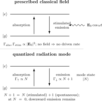
A prescribed classical field drives absorption and stimulated emission with rates proportional to its intensity. For a quantized mode, absorption is proportional to $N$, while emission is proportional to $N+1$. The $N$ part is stimulated emission; the remaining $1$ survives in vacuum and produces spontaneous emission when a continuum of final photon modes is available.

Mode-Resolved Quantum Rates

Consider a lower matter state $\lvert g\rangle$, an upper state $\lvert e\rangle$, and

$$E_e-E_g = \hbar\omega_0.$$

For a mode $(\mathbf k,\lambda)$, absorption changes

$$\lvert g;N_{\mathbf k\lambda}\rangle \longrightarrow \lvert e;N_{\mathbf k\lambda}-1\rangle.$$

Its squared interaction matrix element is

$$\begin{aligned} \lvert M_{\mathrm{abs}}\rvert^2 ={}& \frac{\hbar\omega_{\mathbf k}} {2\epsilon_0\mathcal V} N_{\mathbf k\lambda} \\ &\times \left| \mathbf d_{eg}\cdot \boldsymbol\epsilon_{\mathbf k\lambda} \right|^2. \end{aligned}$$

Emission changes

$$\lvert e;N_{\mathbf k\lambda}\rangle \longrightarrow \lvert g;N_{\mathbf k\lambda}+1\rangle,$$

with

$$\begin{aligned} \lvert M_{\mathrm{em}}\rvert^2 ={}& \frac{\hbar\omega_{\mathbf k}} {2\epsilon_0\mathcal V} (N_{\mathbf k\lambda}+1) \\ &\times \left| \mathbf d_{ge}\cdot \boldsymbol\epsilon_{\mathbf k\lambda}^* \right|^2. \end{aligned}$$

The corresponding golden-rule expressions are

$$\begin{aligned} \Gamma_{g\to e}^{(\mathbf k\lambda)} ={}& \frac{2\pi}{\hbar} \lvert M_{\mathrm{abs}}\rvert^2 \\ &\times \delta(E_e-E_g-\hbar\omega_{\mathbf k}), \end{aligned}$$

and

$$\begin{aligned} \Gamma_{e\to g}^{(\mathbf k\lambda)} ={}& \frac{2\pi}{\hbar} \lvert M_{\mathrm{em}}\rvert^2 \\ &\times \delta(E_e-E_g-\hbar\omega_{\mathbf k}). \end{aligned}$$

Splitting

$$N+1 = \underbrace{N}_{\text{stimulated}} + \underbrace{1}_{\text{spontaneous}}$$

is physically meaningful here:

• the term proportional to $N$ is stimulated emission into an occupied mode;
• the remaining term is spontaneous emission into that mode;
• absorption has no vacuum term because $a\lvert0\rangle=0$.

The vacuum contribution should not be pictured as an ordinary photon already present in the mode. It follows from the quantum field’s operator algebra and the availability of a final one-photon state.

Single mode versus continuum

The golden-rule delta function is not reliable for a perfectly isolated atom coupled to one exactly resonant lossless mode. That problem can show coherent excitation exchange and belongs to the Jaynes–Cummings Model. Irreversible exponential decay emerges when many modes form an effectively continuous reservoir and the return amplitude can be neglected over the time window of interest.

Free-Space Spontaneous Emission

Set all photon occupations to zero and sum the mode-resolved emission rate over free-space wavevectors and polarizations. The continuum replacement is

$$\sum_{\mathbf k} \longrightarrow \frac{\mathcal V}{(2\pi)^3} \int_0^\infty k^2dk \int d\Omega.$$

The factor $1/\mathcal V$ in the squared mode field cancels the $\mathcal V$ in the mode density. For transverse polarizations,

$$\sum_{\lambda=1}^{2} \left| \mathbf d_{ge}\cdot \boldsymbol\epsilon_{\mathbf k\lambda} \right|^2 = \lvert\mathbf d_{ge}\rvert^2 - \left| \mathbf d_{ge}\cdot\widehat{\mathbf k} \right|^2.$$

The differential free-space rate is

$$\begin{aligned} \frac{d\Gamma_0}{d\Omega} ={}& \frac{\omega_0^3} {8\pi^2\epsilon_0\hbar c^3} \\ &\times \left( \lvert\mathbf d_{ge}\rvert^2 - \left| \mathbf d_{ge}\cdot\widehat{\mathbf k} \right|^2 \right). \end{aligned}$$

Integrating over direction gives the standard electric-dipole rate

$$\Gamma_0 = \frac{ \omega_0^3 \lvert\mathbf d_{ge}\rvert^2 }{ 3\pi\epsilon_0\hbar c^3 }.$$

This formula assumes:

• free space in three spatial dimensions;
• electric-dipole coupling;
• weak atom–field coupling;
• a continuum of photon modes;
• Markov or Wigner–Weisskopf behavior over the decay window;
• no boundaries, cavities, waveguides, or material dispersion;
• a fixed transition dipole rather than an unresolved degenerate multiplet.

The $\omega_0^3$ scaling combines the electromagnetic mode density with the frequency dependence of the vacuum electric field per photon. The same normalization cancellation is a concrete application of Density of States in Transition Rates.

Lifetime, branching, and natural width

If an upper state can decay to several lower states,

$$\Gamma_e = \sum_g\Gamma_{e\to g}.$$

Its radiative lifetime is

$$\tau_e = \frac{1}{\Gamma_e},$$

and the branching fraction into channel $g$ is

$$b_{e\to g} = \frac{\Gamma_{e\to g}}{\Gamma_e}.$$

In the ideal Markov model, the excited amplitude and population behave as

$$c_e(t) \propto e^{-\Gamma_e t/2}, \qquad P_e(t) = e^{-\Gamma_e t}.$$

The corresponding lifetime-limited Lorentzian has angular-frequency full width at half maximum $\Gamma_e$. Real spectra can also contain Doppler, collisional, power, transit-time, and inhomogeneous broadening. Those mechanisms should not be folded into $\Gamma_e$ without a model.

Structured electromagnetic environments

Cavities, waveguides, interfaces, photonic crystals, and absorptive media change the available mode density and field profiles. The replacement

$$\Gamma_0 \longrightarrow \Gamma(\mathbf r,\omega_0)$$

can change the total rate, radiation pattern, polarization, branching ratios, and Markov validity. The free-space formula is therefore a benchmark, not a universal law for every photonic environment.

The Quantum Optical Master Equation owns the reduced density-operator dynamics and its assumptions. Thermal and Vacuum Noise owns the bath-correlation viewpoint.

Thermal and Occupied Radiation Modes

For an equilibrium bosonic radiation bath,

$$\overline n(\omega,T) = \frac{1}{e^{\beta\hbar\omega}-1}.$$

Under the same weak-coupling and Markov assumptions used for $\Gamma_0$, the two-level rates are

$$\Gamma_\downarrow = \Gamma_0 [\overline n(\omega_0,T)+1],$$

and

$$\Gamma_\uparrow = \Gamma_0 \overline n(\omega_0,T).$$

Their ratio is

$$\frac{\Gamma_\uparrow} {\Gamma_\downarrow} = e^{-\beta\hbar\omega_0}.$$

At zero temperature, $\overline n=0$: upward thermal excitation vanishes, while downward spontaneous emission remains. At high thermal occupation, the $+1$ becomes negligible compared with $\overline n$, and upward and downward stimulated rates become nearly equal.

Einstein Coefficient Bridge

Spectroscopy and laser physics often package the same physics into Einstein coefficients. For lower and upper levels $g$ and $e$, write

$$R_{g\to e} = B_{ge}\,u(\omega_0),$$

and

$$R_{e\to g} = A_{eg} + B_{eg}\,u(\omega_0).$$

Here $u(\omega)$ is the total isotropic radiation energy density per unit angular frequency. With this convention, thermal equilibrium implies

$$g_gB_{ge} = g_eB_{eg},$$

where $g_g$ and $g_e$ are level degeneracies, and

$$\frac{A_{eg}}{B_{eg}} = \frac{\hbar\omega_0^3} {\pi^2c^3}.$$

Factors of $2\pi$, degeneracies, polarization averages, and line-profile normalizations change when one uses energy density per ordinary frequency, per angular frequency, per solid angle, or per polarization. An Einstein coefficient should never be quoted without its spectral-density convention.

The microscopic identifications are:

Einstein language	Microscopic content
$A_{eg}$	vacuum $+1$ term summed over final photon modes
$B_{eg}u$	stimulated emission from occupied modes
$B_{ge}u$	absorption from occupied modes
degeneracy relation	state counting plus microscopic reversibility

This page uses the coefficients only as a bridge. Einstein Coefficients owns their detailed-balance derivation, blackbody connection, spectral-density conventions, and spectroscopic conversion ledger.

Selection Rules, Polarization, and Degeneracy

For electric-dipole transitions, $\mathbf d$ is a rank-$1$ tensor and is odd under parity. In the usual angular-momentum basis, the leading rules are

$$\Delta J=0,\pm1, \qquad J=0\not\leftrightarrow J'=0,$$ $$\Delta M=q, \qquad q=0,\pm1,$$

and opposite initial and final parity.

The polarization selects the spherical component $q$. Relative to a chosen quantization axis:

Polarization component	Addressed dipole component	Magnetic rule
linear along the axis	$q=0$	$\Delta M=0$
one circular component	$q=+1$	$\Delta M=+1$
opposite circular component	$q=-1$	$\Delta M=-1$

The labels $\sigma^+$ and $\sigma^-$ depend on propagation and handedness conventions. The invariant statement is the spherical component $q$ and the matrix element it selects.

For unresolved initial and final magnetic sublevels, a polarization-resolved line strength may involve

$$\begin{aligned} S_{i\to f}^{(\boldsymbol\epsilon)} ={}& \frac{1}{g_i} \sum_{m_i,m_f} \\ &\times \left| \langle f,m_f\rvert \mathbf d\cdot\boldsymbol\epsilon \lvert i,m_i\rangle \right|^2. \end{aligned}$$

The average over initially populated sublevels and the sum over unresolved final sublevels must match the experiment. The Wigner–Eckart theorem separates reduced matrix elements from angular coefficients, but the canonical derivation remains at Dipole Transitions.

An electric-dipole-forbidden line is not absolutely impossible. Magnetic-dipole, electric-quadrupole, two-photon, relativistic, hyperfine-mixing, or symmetry-breaking mechanisms can contribute at higher or different order.

Worked Scale Estimate

Take an optical transition with

$$\lambda_0=500\,\mathrm{nm}$$

and a transition dipole of one atomic unit,

$$\lvert\mathbf d_{ge}\rvert = ea_0 \approx 8.48\times10^{-30}\,\mathrm{C\,m}.$$

The angular frequency is

$$\omega_0 = \frac{2\pi c}{\lambda_0} \approx 3.77\times10^{15}\,\mathrm{s^{-1}}.$$

The free-space electric-dipole estimate is

$$\Gamma_0 \approx 1.62\times10^7\,\mathrm{s^{-1}}.$$

Thus

$$\tau \approx 6.17\times10^{-8}\,\mathrm{s} = 61.7\,\mathrm{ns},$$

and the lifetime-limited width in ordinary frequency is

$$\frac{\Gamma_0}{2\pi} \approx 2.58\,\mathrm{MHz}.$$

This is an order-of-magnitude example, not a prediction for a named line. Real rates depend on the actual many-electron or molecular matrix element, angular factors, branching channels, environment, and nonradiative decay.

What a Measured Spectral Line Contains

A measured line should not be identified with a bare golden-rule matrix element. Its interpretation typically combines:

Observable feature	Main theoretical ingredients
center frequency	energy difference plus shifts
integrated strength	matrix element, populations, degeneracy, geometry
line shape	pulse envelope, lifetime, motion, collisions, environment
polarization	tensor component and experimental axis conventions
emitted intensity	upper-state population, rate, branching, collection efficiency
absorbed intensity	lower-state population, optical depth, propagation, saturation

The historical and instrumental meaning of these quantities belongs to Spectroscopy. Saturation and steady-state driven dynamics belong to the Optical Bloch Equations.

Regime Map

Physical situation	Appropriate starting description
weak finite classical pulse	first-order transition amplitude
weak drive into a dense continuum	golden-rule absorption or stimulated rate
strong or long resonant drive of one transition	Rabi dynamics
atom coupled coherently to one lossless cavity mode	Rabi or Jaynes–Cummings model
excited atom radiating into many vacuum modes	spontaneous-emission continuum calculation
driven atom with decay and dephasing	optical Bloch equations
structured photonic reservoir	environment-specific mode density or Green tensor
higher-multipole or forbidden transition	M1, E2, two-photon, or mixed-state treatment

The choice is controlled by mode density, coupling strength, observation time, occupation, and coherence—not merely by whether the process is called optical.

Calculation Workflow

1. Solve the matter problem: identify $E_i$, $E_f$, and the good quantum numbers.
2. Choose the interaction: minimal coupling, electric dipole, or a higher multipole.
3. State the field model: prescribed classical wave, pulse, one quantized mode, or continuum reservoir.
4. Fix normalization: peak field versus rms field, intensity, mode volume, and delta-function convention.
5. Project polarization: evaluate $\boldsymbol\epsilon\cdot\mathbf d_{fi}$ in a declared axis convention.
6. Apply symmetry: remove forbidden channels before numerical integration.
7. Choose probability or rate: verify that a continuum and intermediate-time rate window exist.
8. Sum and average correctly: include final channels, initial populations, degeneracies, directions, and polarizations.
9. Audit dynamics: check depletion, saturation, recurrences, damping, and environmental structure.
10. Connect to observables: distinguish line position, integrated strength, width, branching, and detector response.

Common Mistakes

• Dropping the factor $1/2$ when decomposing a real monochromatic field.
• Confusing peak electric-field amplitude with rms amplitude or intensity.
• Writing $\lvert\mathbf d_{fi}\rvert^2$ when the experiment selects one polarization projection.
• Treating resonance as sufficient when the transition matrix element vanishes.
• Calling a finite-time sinc profile a lifetime-broadened Lorentzian.
• Using a golden-rule rate for one isolated lossless resonant mode.
• Expecting a prescribed classical field to derive spontaneous emission.
• Saying that the vacuum contains an ordinary photon that is absorbed or emitted.
• Forgetting the $+1$ in downward bosonic rates or incorrectly adding it to absorption.
• Leaving the photon mode normalization volume in the final free-space rate.
• Applying the free-space $\omega^3$ law inside a cavity or structured medium without modification.
• Quoting Einstein $A$ and $B$ relations without a spectral-density convention.
• Averaging over magnetic sublevels or polarizations differently from the experimental preparation and detection.
• Equating a radiative lifetime with the measured lifetime when nonradiative channels exist.
• Treating electric-dipole forbidden as absolutely forbidden.

Exercises

1. Recover the semiclassical absorption factor

For

$$\mathbf E(t) = \mathcal E_0 \boldsymbol\epsilon \cos\omega t$$

with real $\mathcal E_0$ and $\boldsymbol\epsilon$, derive the golden-rule absorption rate in angular-frequency delta-function form.

Solution

Decompose the cosine:

$$\cos\omega t = \frac12 \left( e^{-i\omega t}+e^{i\omega t} \right).$$

The resonant absorption operator is

$$W = -\frac{\mathcal E_0}{2} \mathbf d\cdot\boldsymbol\epsilon.$$

Therefore

$$\begin{aligned} \Gamma_{i\to f}^{\mathrm{abs}} ={}& \frac{2\pi}{\hbar} \frac{\mathcal E_0^2}{4} \left| \boldsymbol\epsilon\cdot\mathbf d_{fi} \right|^2 \\ &\times \delta(E_f-E_i-\hbar\omega). \end{aligned}$$

Since

$$\delta(E_f-E_i-\hbar\omega) = \frac{1}{\hbar} \delta(\omega_{fi}-\omega),$$

the result is

$$\begin{aligned} \Gamma_{i\to f}^{\mathrm{abs}} ={}& \frac{\pi\mathcal E_0^2}{2\hbar^2} \left| \boldsymbol\epsilon\cdot\mathbf d_{fi} \right|^2 \\ &\times \delta(\omega-\omega_{fi}). \end{aligned}$$

The factor $1/4$ in the squared matrix element comes from the two $1/2$ factors in the harmonic amplitude.

2. Derive the occupation factors

Show that absorption from a mode with $N$ photons is proportional to $N$, whereas emission into that mode is proportional to $N+1$.

Solution

Absorption annihilates one photon:

$$\langle N-1\rvert a\lvert N\rangle = \sqrt N.$$

Squaring gives the factor $N$. Emission creates one photon:

$$\langle N+1\rvert a^\dagger\lvert N\rangle = \sqrt{N+1}.$$

Squaring gives $N+1$. At $N=0$, absorption vanishes while emission remains possible.

3. Integrate the dipole radiation pattern

Take a real transition dipole along $z$. Use the differential rate to recover the total free-space spontaneous-emission rate.

Solution

For $\mathbf d=d\widehat{\mathbf z}$,

$$\lvert\mathbf d\rvert^2 - \lvert\mathbf d\cdot\widehat{\mathbf k}\rvert^2 = d^2\sin^2\theta.$$

The angular integral is

$$\begin{aligned} \int d\Omega\,\sin^2\theta &= 2\pi \int_0^\pi d\theta\,\sin^3\theta \\ &= \frac{8\pi}{3}. \end{aligned}$$

Therefore

$$\begin{aligned} \Gamma_0 &= \frac{\omega_0^3d^2} {8\pi^2\epsilon_0\hbar c^3} \frac{8\pi}{3} \\ &= \frac{\omega_0^3d^2} {3\pi\epsilon_0\hbar c^3}. \end{aligned}$$

4. Check thermal detailed balance

Starting from $\Gamma_\downarrow=\Gamma_0(\overline n+1)$ and $\Gamma_\uparrow=\Gamma_0\overline n$, show that their ratio is the Boltzmann factor.

Solution

For a Bose–Einstein occupation,

$$\overline n = \frac{1}{e^{\beta\hbar\omega_0}-1}.$$

Then

$$\overline n+1 = \frac{e^{\beta\hbar\omega_0}} {e^{\beta\hbar\omega_0}-1}.$$

Hence

$$\frac{\Gamma_\uparrow} {\Gamma_\downarrow} = \frac{\overline n}{\overline n+1} = e^{-\beta\hbar\omega_0}.$$

5. Resolve polarization-selected sublevels

An electric-dipole transition begins in $J_i=0$, $M_i=0$ and ends in a $J_f=1$ multiplet. Which final magnetic sublevel is addressed by each spherical polarization component $q=0,+1,-1$?

Solution

The electric-dipole magnetic rule is

$$M_f=M_i+q.$$

Since $M_i=0$,

$$q=0\Rightarrow M_f=0,$$ $$q=+1\Rightarrow M_f=+1,$$

and

$$q=-1\Rightarrow M_f=-1.$$

All three are allowed by angular momentum, but a field with one definite spherical polarization addresses only its matching component in this idealized geometry.

6. Compute a lifetime and branching fractions

An excited level has three independent radiative decay channels with rates

$$\Gamma_1=2.0\times10^6\,\mathrm{s^{-1}},$$ $$\Gamma_2=3.0\times10^6\,\mathrm{s^{-1}},$$

and

$$\Gamma_3=5.0\times10^6\,\mathrm{s^{-1}}.$$

Find the lifetime and branching fractions. State one reason the measured lifetime could be shorter.

Solution

The total radiative rate is

$$\Gamma_e = \Gamma_1+\Gamma_2+\Gamma_3 = 1.0\times10^7\,\mathrm{s^{-1}}.$$

Thus

$$\tau_e = \frac{1}{\Gamma_e} = 1.0\times10^{-7}\,\mathrm s = 100\,\mathrm{ns}.$$

The branching fractions are

$$\begin{gathered} b_1=0.20, \qquad b_2=0.30, \\ b_3=0.50. \end{gathered}$$

A nonradiative decay channel, collisional quenching, or an environment-enhanced radiative channel would add to the total decay rate and shorten the measured lifetime.

Cross-Links

• Time-Dependent Perturbation Theory and Transitions
• Harmonic Perturbations
• Resonant Driving
• Einstein Coefficients
• Fermi’s Golden Rule
• Density of States in Transition Rates
• Selection Rules in Transition Rates
• Linear Response Preview
• Minimal Coupling in Wave Mechanics
• Dipole Approximation
• Dipole Transitions
• Multipole Operators
• Spontaneous Emission
• Quantum Optical Master Equation
• Optical Bloch Equations
• Thermal and Vacuum Noise
• Spectroscopy Chapter Overview
• Transition Rates
• Spectroscopy as an Experimental Technique
• Light-Matter Models

References

• P. A. M. Dirac, “The quantum theory of the emission and absorption of radiation,” Proceedings of the Royal Society A 114, 243–265 (1927), doi:10.1098/rspa.1927.0039.
• V. Weisskopf and E. Wigner, “Berechnung der natürlichen Linienbreite auf Grund der Diracschen Lichttheorie,” Zeitschrift für Physik 63, 54–73 (1930), doi:10.1007/BF01336768.
• C. Cohen-Tannoudji, J. Dupont-Roc, and G. Grynberg, Atom–Photon Interactions: Basic Processes and Applications, Wiley, 1992.
• M. O. Scully and M. S. Zubairy, Quantum Optics, Cambridge University Press, 1997.
• C. J. Foot, Atomic Physics, Oxford University Press, 2005.
• R. D. Cowan, The Theory of Atomic Structure and Spectra, University of California Press, 1981.
• National Institute of Standards and Technology, Atomic Spectra Database: Spectral Lines Help, transition probabilities, oscillator strengths, and line-strength conventions.