Dipole Approximation

The electric-dipole approximation replaces the variation of an electromagnetic mode across a localized internal charge distribution by its value at one reference point. For a neutral atom or molecule, the leading internal coupling is then

$$H_{E1}(t) = - \mathbf d \mathbin{\cdot} \mathbf E(\mathbf R,t).$$

This compact Hamiltonian underlies much of spectroscopy, laser control, quantum optics, and atomic-clock physics. Its familiarity can hide several independent assumptions. In particular:

• it is a spatial approximation, not a weak-field approximation;
• it can be valid for internal motion while the center-of-mass phase $e^{i\mathbf k\cdot\mathbf R}$ remains essential;
• it does not imply that electric-dipole coupling is the leading nonzero transition amplitude;
• it does not by itself justify a two-level truncation, perturbation theory, a rotating-wave approximation, or a classical treatment of light.

The reliable question is therefore not merely “is the wavelength larger than the atom?” It is “which field gradients are resolved by the charge or current matrix element relevant to this observable?”

Canonical Scope

This page owns the long-wavelength reduction used in atomic, molecular, and optical physics:

1. expanding a field or mode function about a reference point;
2. obtaining the electric-dipole Hamiltonian;
3. defining and interpreting transition dipole moments;
4. separating internal, center-of-mass, beam-profile, and motional scales;
5. deciding when magnetic-dipole, electric-quadrupole, or full spatial coupling must be retained.

The parent many-charge Hamiltonian, including the $A^2$ term, lives in Minimal Coupling. The relation among length, velocity, and multipolar representations lives in Gauge Choices in Light–Matter Physics.

This page does not repeat the angular-momentum and parity derivation of E1 selection rules. That is the canonical subject of Dipole Transitions. Rates and lineshapes begin only after an interaction matrix element has been chosen; see Transition Rates in Light–Matter Interaction.

Coordinates and Conventions

Let the constituents have charges $q_a$ and positions

$$\mathbf x_a = \mathbf R+\boldsymbol\rho_a.$$

Here $\mathbf R$ is an expansion point, often the center of mass, a nucleus, or a fixed molecular origin, and $\boldsymbol\rho_a$ is an internal coordinate relative to it. Define

$$Q = \sum_a q_a, \qquad \mathbf d = \sum_a q_a\boldsymbol\rho_a.$$

Most optical applications on this page concern a localized neutral system, $Q=0$. Charged systems require more care because uniform electric fields also accelerate the center of mass and because a permanent dipole depends on the choice of origin.

Repeated Cartesian indices are summed when an index form is used. The electric field is a real field unless a complex amplitude is displayed explicitly. The sign convention

$$H_{E1} = - \mathbf d\mathbin{\cdot}\mathbf E$$

then follows from the potential energy of a charge distribution in an external electric field.

Long-Wavelength Approximation

Taylor expansion of a smooth field

Suppose the field is smooth over the support of the internal wavefunction. For each constituent,

$$\begin{aligned} E_j( \mathbf R+\boldsymbol\rho_a,t ) ={}& E_j(\mathbf R,t) \\ &+ \rho_{a,i} \partial_i E_j(\mathbf R,t) \\ &+ \frac{1}{2} \rho_{a,i}\rho_{a,k} \partial_i\partial_k E_j(\mathbf R,t) \\ &+ \cdots. \end{aligned}$$

Keeping only the first line makes the field uniform across the internal coordinates. It need not make the field uniform over the apparatus or over a center-of-mass trajectory.

For a plane-wave component,

$$\mathbf E( \mathbf R+\boldsymbol\rho,t ) \propto \boldsymbol\epsilon e^{i\mathbf k\cdot\mathbf R} e^{i\mathbf k\cdot\boldsymbol\rho} e^{-i\omega t}.$$

The internal spatial factor has the expansion

$$\begin{aligned} e^{i\mathbf k\cdot\boldsymbol\rho} ={}& 1 + i\mathbf k\mathbin{\cdot}\boldsymbol\rho \\ &- \frac{1}{2} \left( \mathbf k\mathbin{\cdot}\boldsymbol\rho \right)^2 + \cdots. \end{aligned}$$

If $a$ is a characteristic internal extent, the conventional long-wavelength parameter is

$$\eta_{\mathrm{int}} = ka = \frac{2\pi a}{\lambda}.$$

The leading internal replacement is controlled when $\eta_{\mathrm{int}}\ll1$. The factor of $2\pi$ matters: the comparison is with the reduced wavelength $1/k$, not merely with $\lambda$.

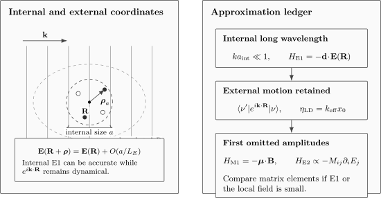
The internal approximation tests variation over $\boldsymbol\rho$, while the phase at $\mathbf R$ can still drive recoil, Doppler shifts, and motional sidebands. When E1 is suppressed, compare actual M1 and E2 matrix elements rather than relying on the nominal $ka$ hierarchy.

What size should enter ka?

A geometric radius is only a first estimate. The relevant object is the charge or current transition distribution, not necessarily the full diameter of the system. Define the charge-density operator

$$\widehat\rho_q(\mathbf x) = \sum_a q_a \delta^{(3)} \left( \mathbf x-\mathbf x_a \right)$$

and its transition density

$$\rho_{fi}(\mathbf x) = \langle f| \widehat\rho_q(\mathbf x) |i\rangle.$$

An optional diagnostic length is

$$a_{fi}^2 = \frac{ \displaystyle \int d^3x\, |\mathbf x-\mathbf R|^2 |\rho_{fi}(\mathbf x)| }{ \displaystyle \int d^3x\, |\rho_{fi}(\mathbf x)| }.$$

This absolute-density definition is a scale estimate, not a unique observable. A more decisive test is to calculate the first omitted interaction matrix element and compare it with the retained one.

This distinction matters in X-ray spectroscopy. A molecule may be several ångströms across while a particular core transition density is concentrated near one nucleus. Conversely, a Rydberg or continuum state can sample a much larger region than the ground-state radius suggests.

General modes and near fields

For a cavity mode, focused beam, evanescent wave, or near field, $1/k$ may not be the shortest spatial scale. A local gradient length can be defined schematically by

$$\frac{1}{L_E} \sim \frac{ \|\boldsymbol\nabla\mathbf E\| }{ E_{\mathrm{ref}} },$$

where $E_{\mathrm{ref}}$ is a nonzero field scale appropriate to the experiment. The corresponding estimate is

$$\epsilon_{\mathrm{grad}} \sim \frac{a}{L_E}.$$

At a node, using the local $|\mathbf E(\mathbf R)|$ as the denominator is meaningless because it vanishes. One must compare the gradient-driven and field-driven matrix elements directly. Structured light can therefore make beyond-dipole coupling leading even when $ka$ is very small.

Choosing the Expansion Point

Neutral and charged systems

Shift the reference point by a fixed vector $\mathbf s$:

$$\mathbf R' = \mathbf R+\mathbf s, \qquad \boldsymbol\rho_a' = \boldsymbol\rho_a-\mathbf s.$$

The dipole operator transforms as

$$\mathbf d' = \mathbf d-Q\mathbf s.$$

For a neutral system, $\mathbf d'=\mathbf d$ as an operator. For a charged system, the permanent dipole is origin dependent. However, between distinct orthonormal states in the same charge sector,

$$\begin{aligned} \mathbf d_{fi}' &= \langle f|\mathbf d'|i\rangle \\ &= \mathbf d_{fi} - Q\mathbf s\, \langle f|i\rangle \\ &= \mathbf d_{fi}, \qquad f\ne i. \end{aligned}$$

Thus an off-diagonal transition dipole is origin independent under a fixed shift, even for a charged system. Diagonal moments and center-of-mass couplings still require the charge and origin to be stated.

Higher multipoles mix under shifts

Beyond E1, shifting the expansion point redistributes contributions among multipole orders and changes the plane-wave phase. An exact, untruncated interaction is independent of that bookkeeping. A truncated expression is origin independent only when all terms required at the claimed order are kept consistently.

This is especially important for oscillator strengths beyond the dipole approximation. Keeping the square of an E2 or M1 amplitude while dropping interference terms of the same order can create spurious origin dependence.

Useful choices

• Neutral atom: a nucleus or the center of mass gives compact internal coordinates.
• Ion: the center of mass supports a clean separation of internal and external motion.
• Centrosymmetric molecule: the inversion center makes parity labels transparent.
• General molecule: the center of mass or a fixed molecular origin makes multipoles reproducible.
• Localized core excitation: the absorbing nucleus can make a local expansion efficient.
• Trapped particle: the equilibrium trap position plus a position operator exposes the motional phase.

The best origin is the one that matches the symmetry and scale separation, not the one that makes one selected term look smallest.

Electric Dipole Hamiltonian

Multipolar form

For a localized neutral system in a smooth external field, the leading internal term in the multipolar expansion is

$$H_{E1}(t) = - \mathbf d \mathbin{\cdot} \mathbf E(\mathbf R,t).$$

This is often called the length-form interaction. It arises naturally in the Power–Zienau–Woolley representation. Starting in a velocity or minimal-coupling representation, one first replaces the vector potential by its value over the internal coordinates and then performs the corresponding unitary transformation. “Dipole approximation” and “length gauge” are therefore related but not logically identical statements.

For a charged composite system, the complete long-wavelength Hamiltonian also contains center-of-mass coupling to the monopole charge. Writing only $-\mathbf d\cdot\mathbf E$ silently discards that dynamics.

Classical field convention

For a monochromatic classical field, write

$$\mathbf E(\mathbf R,t) = \frac{1}{2} \left[ \boldsymbol{\mathcal E}(\mathbf R) e^{-i\omega t} + \boldsymbol{\mathcal E}^{*}(\mathbf R) e^{i\omega t} \right].$$

Then

$$\begin{aligned} H_{E1}(t) ={}& - \frac{1}{2} \mathbf d\mathbin{\cdot} \boldsymbol{\mathcal E}(\mathbf R) e^{-i\omega t} \\ &- \frac{1}{2} \mathbf d\mathbin{\cdot} \boldsymbol{\mathcal E}^{*}(\mathbf R) e^{i\omega t}. \end{aligned}$$

The factor $1/2$ belongs to this complex-amplitude convention. If $\boldsymbol{\mathcal E}$ is instead defined as a positive-frequency field without the usual real-field decomposition, the factor changes. Many apparent factor-of-two disagreements in Rabi frequencies are convention disagreements.

Quantized field

For orthonormal transverse modes $\mathbf f_\lambda(\mathbf r)$, one common normalization gives

$$\begin{aligned} \widehat{\mathbf E}_{\perp}(\mathbf R) ={}& i \sum_\lambda \sqrt{ \frac{ \hbar\omega_\lambda }{ 2\epsilon_0 } } \\ &\times \left[ \mathbf f_\lambda(\mathbf R) \widehat a_\lambda - \mathbf f_\lambda^*(\mathbf R) \widehat a_\lambda^\dagger \right]. \end{aligned}$$

The dipole interaction is then

$$\widehat H_{E1} = - \widehat{\mathbf d} \mathbin{\cdot} \widehat{\mathbf E}_{\perp}(\mathbf R).$$

Mode normalization may place a quantization volume or effective mode volume inside $\mathbf f_\lambda$. A single-mode coupling is often defined by

$$\hbar g_{fi} = - \mathbf d_{fi} \mathbin{\cdot} \mathbf E_{\mathrm{vac}}(\mathbf R),$$

up to a phase convention. The same long-wavelength test applies to the mode function: it must vary little over the internal transition distribution.

In a fully quantized multipolar Hamiltonian, polarization self-energy terms belong to the same transformed theory. The dipole approximation is not a license to delete them. Their role and the gauge dependence of finite-level models are discussed in Gauge Choices in Light–Matter Physics.

Fixed nuclei and molecular coordinates

For electrons at $\mathbf r_j$ and nuclei at $\mathbf R_A$,

$$\begin{aligned} \mathbf d ={}& - e \sum_j \left( \mathbf r_j-\mathbf R \right) \\ &+ e \sum_A Z_A \left( \mathbf R_A-\mathbf R \right). \end{aligned}$$

At fixed nuclear geometry, the nuclear term is proportional to the identity in the electronic Hilbert space and therefore drops from an off-diagonal electronic transition dipole. It does not disappear from permanent dipoles, vibrational transitions, vibronic coupling, or nuclear dynamics.

In the Born–Oppenheimer description, a geometry-dependent electronic dipole surface can couple vibrational states. Infrared intensity is controlled by how the molecular dipole changes along a normal coordinate, not merely by whether the equilibrium molecule has a permanent dipole.

Transition Dipole Moments

Definition

For matter eigenstates $|i\rangle$ and $|f\rangle$, define

$$\mathbf d_{fi} = \langle f|\mathbf d|i\rangle.$$

The E1 matrix element is

$$\langle f| H_{E1}(t) |i\rangle = - \mathbf d_{fi} \mathbin{\cdot} \mathbf E(\mathbf R,t).$$

For a classical complex amplitude, a common Rabi-frequency convention is

$$\Omega_{fi} = - \frac{ \mathbf d_{fi} \mathbin{\cdot} \boldsymbol{\mathcal E}(\mathbf R) }{ \hbar }.$$

With the real-field convention above, the resonant rotating-wave Hamiltonian contains $\hbar\Omega_{fi}/2$. A transition rate requires additional assumptions about time dependence, density of final states, field statistics, and line broadening.

Transition density interpretation

The same matrix element can be written

$$\mathbf d_{fi} = \int d^3x\, \left( \mathbf x-\mathbf R \right) \rho_{fi}(\mathbf x).$$

For distinct states in one charge sector,

$$\int d^3x\, \rho_{fi}(\mathbf x) = Q\langle f|i\rangle = 0.$$

The transition density therefore carries no net transition charge. The transition dipole is its first spatial moment. Positive and negative regions can cancel strongly, so a large spatial extent does not guarantee a large dipole matrix element.

Permanent and transition dipoles are different

The diagonal quantity

$$\mathbf d_{ii} = \langle i|\mathbf d|i\rangle$$

is a permanent-state dipole. The off-diagonal quantity $\mathbf d_{fi}$ is a transition dipole. A state can have zero permanent dipole and still have strong E1 transitions. Conversely, a polar molecule can have a nonzero permanent dipole while a particular transition dipole vanishes.

Polarization projection

For a mode with polarization $\boldsymbol\epsilon$, only

$$d_{fi}^{(\epsilon)} = \boldsymbol\epsilon \mathbin{\cdot} \mathbf d_{fi}$$

enters the E1 amplitude. The vector can be complex when the states or polarization basis are complex. Observable strengths involve absolute squares and, where appropriate, sums or averages over magnetic sublevels and polarizations.

The rotational and parity conditions under which this projection vanishes belong to Dipole Transitions. “Allowed” means not forced to zero by the stated symmetry; it does not mean large.

Degenerate subspaces

Within a degenerate manifold, individual vectors $\mathbf d_{fi}$ depend on the chosen basis. A physical preparation, field polarization, external splitting, or incoherent average selects the relevant combination. Summing over a complete unresolved degenerate manifold produces a basis-independent strength, while quoting one arbitrarily chosen component may not.

Length and velocity matrix elements

For a local nonrelativistic Hamiltonian

$$H_0 = \frac{\mathbf p^2}{2m} + V(\mathbf r),$$

the commutator

$$[H_0,\mathbf r] = - \frac{i\hbar}{m} \mathbf p$$

implies, for exact eigenstates,

$$\mathbf p_{fi} = im\omega_{fi} \mathbf r_{fi}.$$

This relation makes exact length- and velocity-form E1 amplitudes equivalent when all terms are treated consistently. Incomplete bases, nonlocal pseudopotentials, inconsistent energies, or omitted contact terms can spoil the numerical agreement. That disagreement is a convergence diagnostic, not a physical gauge dependence.

Validity Conditions

Internal spatial variation

The first check is

$$k a_{fi} \ll 1$$

for every appreciably occupied spectral component and for the transition distribution of interest. For a broadband pulse, use the largest relevant $k$, not only the carrier wave number.

For a general field, also check

$$a_{fi} \frac{ \|\boldsymbol\nabla\mathbf E\| }{ E_{\mathrm{ref}} } \ll 1, \qquad a_{fi}^2 \frac{ \|\boldsymbol\nabla\boldsymbol\nabla\mathbf E\| }{ E_{\mathrm{ref}} } \ll 1.$$

These estimates test the expansion, not the dominance of a particular transition.

Transition-specific amplitude test

When the E1 amplitude is nonzero, the most useful diagnostic is

$$\epsilon_{fi}^{(1)} = \frac{ \left| \langle f|H_{\mathrm{M1}}+H_{\mathrm{E2}}|i\rangle \right| }{ \left| \langle f|H_{\mathrm{E1}}|i\rangle \right| }.$$

If the denominator vanishes or is accidentally small, this ratio is not a failure of arithmetic. It says that E1 is not the reference process. Compare each candidate amplitude with the largest retained physical amplitude instead.

Center-of-mass phase is a separate approximation

After making the internal dipole approximation, a plane-wave interaction still contains

$$H_{E1} \propto - \mathbf d \mathbin{\cdot} \boldsymbol\epsilon\, e^{i\mathbf k\cdot\mathbf R}.$$

The factor $e^{i\mathbf k\cdot\mathbf R}$ transfers photon momentum and couples center-of-mass motional states. Removing it requires a second approximation about the external wavepacket or trajectory.

For motional states $|\nu\rangle$,

$$\langle \nu'| e^{i\mathbf k\cdot\mathbf R} |\nu\rangle$$

sets carrier and sideband strengths. In one harmonic direction with

$$x_0 = \sqrt{ \frac{\hbar}{2M\omega_t} },$$

the Lamb–Dicke parameter is

$$\eta_{\mathrm{LD}} = k_{\mathrm{eff}}x_0.$$

A useful state-dependent condition is

$$\eta_{\mathrm{LD}} \sqrt{2\bar n+1} \ll 1.$$

The effective wave vector is $\mathbf k$ for a one-photon process and often a wave-vector difference for a Raman process. It is entirely possible to have

$$k a_{\mathrm{int}} \ll 1$$

while not being in the Lamb–Dicke regime. The first statement concerns internal electronic or molecular structure; the second concerns external motion.

The recoil energy

$$E_{\mathrm r} = \frac{ \hbar^2k^2 }{ 2M }$$

and the Doppler shift $\mathbf k\cdot\mathbf V$ also survive the internal dipole approximation.

Beam profile and structured light

A paraxial beam introduces transverse and longitudinal scales in addition to $1/k$. For waist $w_0$, a localized internal system usually satisfies $a/w_0\ll1$, but center-of-mass motion may sample the profile. Near a focus, interface, nanostructure, or optical vortex, longitudinal fields and steep gradients can matter.

At an electric-field node, the E1 amplitude can vanish because $\mathbf E(\mathbf R)=0$ even though the E1 transition dipole is symmetry allowed. M1 or E2 coupling may then be the leading local interaction. This is a mode-geometry statement, not an intrinsic atomic selection rule.

Strong fields and changing length scales

The dipole approximation does not require a weak field. Intense-field calculations often use a dipole Hamiltonian nonperturbatively. Nevertheless, the field can drive the wavefunction into Rydberg or continuum regions with a larger spatial extent, making the initial bound-state radius a poor value of $a$.

Strong fields can independently invalidate:

• perturbation theory;
• a two-level reduction;
• the rotating-wave approximation;
• neglect of ionization or continuum states;
• a nonrelativistic treatment;
• a prescribed-field model that ignores depletion or backaction.

None of these failures follows solely from $ka$.

Temporal bandwidth

Spatial and temporal variations are linked for freely propagating radiation through $k=\omega/c$, but the approximation is still made in space. For a pulse with spectral support up to $\omega_{\max}$, a conservative test is

$$\frac{ \omega_{\max}a }{ c } \ll 1.$$

Using only the carrier can miss a high-frequency tail. A short pulse does not otherwise invalidate E1 coupling merely because it is short.

Near fields and material environments

Evanescent and quasistatic fields can have gradient scales set by distance to a surface, aperture size, or nanostructure geometry rather than by the free-space wavelength. The local test is then $a/L_E$, together with direct M1 and E2 matrix-element comparisons.

In periodic systems, a naive unbounded position operator is not generally the right starting point. Current operators, Berry-phase polarization, and the chosen boundary conditions must be handled consistently. The localized atom-and-molecule construction here should not be transplanted unchanged into a crystal.

Worked Scale Estimates

Visible light on a compact atom

Take

$$a=a_0 = 0.0529\ \mathrm{nm}, \qquad \lambda = 500\ \mathrm{nm}.$$

Then

$$\begin{aligned} ka &= \frac{2\pi a_0}{\lambda} \\ &\simeq 6.65\times10^{-4}. \end{aligned}$$

Internal spatial variation is very small. This does not prove that a chosen line is E1 allowed, but it makes the long-wavelength expansion strongly controlled for compact bound-state matrix elements.

Infrared light on a molecule

For

$$a = 0.50\ \mathrm{nm}, \qquad \lambda = 10\ \mathrm{\mu m},$$

one finds

$$ka \simeq 3.14\times10^{-4}.$$

The field is nearly uniform over the molecular framework. Vibrational intensity still depends on the derivative of the molecular dipole surface along the normal coordinate.

X-rays and a localized core transition

For a hard X-ray wavelength

$$\lambda = 0.10\ \mathrm{nm}$$

and a geometric molecular scale $a=0.50\ \mathrm{nm}$,

$$ka \simeq 31.4.$$

A molecular-size dipole approximation is uncontrolled. If the relevant core transition density has an effective extent $a_{fi}=0.02\ \mathrm{nm}$, then

$$k a_{fi} \simeq 1.26,$$

which is smaller but still not asymptotically small. A calculation may need the full spatial interaction rather than a low-order multipole truncation.

Internal dipole regime without Lamb–Dicke confinement

Consider a trapped ion with

$$\lambda = 729\ \mathrm{nm}, \qquad a_{\mathrm{int}} = 0.10\ \mathrm{nm}.$$

The internal parameter is

$$k a_{\mathrm{int}} \simeq 8.62\times10^{-4}.$$

For the actual $^{40}\mathrm{Ca}^{+}$ 729 nm clock transition, the E1 matrix element is forbidden and E2 coupling is leading. The small value of $k a_{\mathrm{int}}$ validates a rapidly ordered internal multipole expansion; it does not promote a vanishing E1 amplitude.

For mass $M=40\,u$ and trap frequency $\omega_t=2\pi\times1.0\ \mathrm{MHz}$,

$$x_0 \simeq 11.2\ \mathrm{nm}, \qquad \eta_{\mathrm{LD}} \simeq 0.0965.$$

The electronic dipole approximation is excellent. At $\bar n=20$,

$$\eta_{\mathrm{LD}} \sqrt{2\bar n+1} \simeq 0.618,$$

so replacing the motional phase by unity is not well controlled. Internal and external long-wavelength statements give different answers because they address different coordinates.

An allowed transition at a standing-wave node

Let

$$\mathbf E(x,t) = \widehat{\mathbf z} E_0 \sin(kx) \cos(\omega t)$$

and place the expansion point at $x=0$. Although the internal parameter can satisfy $ka\ll1$,

$$\mathbf E(0,t) = 0.$$

The local E1 term vanishes. The first electric gradient is

$$\left. \partial_x E_z \right|_{x=0} = kE_0\cos(\omega t),$$

so an electric-quadrupole matrix element can become leading. The standing wave also has a magnetic field, so the M1 amplitude must be checked at the same order.

Breakdown and Multipole Corrections

First omitted interactions

Introduce the primitive electric quadrupole tensor

$$M_{ij} = \sum_a q_a \rho_{a,i}\rho_{a,j}.$$

With this convention, the first terms of a local multipolar interaction can be organized schematically as

$$\begin{aligned} H_{\mathrm{int}} ={}& H_{\mathrm{monopole}}(\mathbf R) - d_i E_i(\mathbf R) \\ &- \mu_i B_i(\mathbf R) - \frac{1}{2} M_{ij} \partial_i E_j(\mathbf R) \\ &+ \cdots. \end{aligned}$$

The magnetic dipole $\boldsymbol\mu$ contains orbital and, where relevant, spin contributions. The displayed formula fixes the primitive-quadrupole normalization used here. For an electrostatic external field, $H_{\mathrm{monopole}}$ includes $Q\Phi(\mathbf R)$. A charged moving system also has center-of-mass vector-potential coupling, so $H_{\mathrm{monopole}}$ is not exhausted by that scalar term.

Alternatively, define a traceless Cartesian quadrupole

$$\Theta_{ij} = \sum_a q_a \left( 3\rho_{a,i}\rho_{a,j} - \rho_a^2\delta_{ij} \right).$$

In a source-free region where $\boldsymbol\nabla\cdot\mathbf E=0$,

$$H_{E2} = - \frac{1}{6} \Theta_{ij} \partial_i E_j(\mathbf R).$$

Factors such as $1/2$ and $1/6$ cannot be compared across references without checking which quadrupole tensor has been defined.

Expected power counting

For a plane wave and typical nonvanishing moments,

$$\frac{ |M_{fi}^{E2}| }{ |M_{fi}^{E1}| } \sim ka.$$

For nonrelativistic internal motion, a typical M1-to-E1 amplitude can scale like $v/c$. In atoms driven near internal resonances, these estimates may be of similar small order. Neither is universal: symmetry, cancellations, relativistic mixing, molecular geometry, and field structure can change the actual ratio.

The hierarchy is a statement about amplitudes. A correction of order $ka$ in amplitude generally contributes at order $ka$ through interference with E1 and at order $(ka)^2$ through its own square, subject to symmetry and orientation averages.

Consistent expansion of probabilities

Write a transition amplitude as

$$\mathcal A = \mathcal A^{(0)} + \mathcal A^{(1)} + \mathcal A^{(2)} + \cdots,$$

where $\mathcal A^{(n)}$ is nominally order $(ka)^n$. Through second order,

$$\begin{aligned} |\mathcal A|^2 ={}& |\mathcal A^{(0)}|^2 \\ &+ 2\operatorname{Re} \left[ \mathcal A^{(0)*} \mathcal A^{(1)} \right] \\ &+ |\mathcal A^{(1)}|^2 \\ &+ 2\operatorname{Re} \left[ \mathcal A^{(0)*} \mathcal A^{(2)} \right] \\ &+ O\!\left((ka)^3\right). \end{aligned}$$

Keeping $|\mathcal A^{(1)}|^2$ while omitting the $\mathcal A^{(0)*}\mathcal A^{(2)}$ interference is not a complete second-order calculation. Such partial truncations can spoil origin independence and sum rules.

When the series is not efficient

If $ka\gtrsim1$, many multipole orders can contribute. In that regime, retaining the exact factor

$$e^{i\mathbf k\cdot\boldsymbol\rho}$$

or the full current–field interaction is often better than extending a slowly convergent multipole series. The exact spatial operator also avoids assigning physical significance to individual origin-dependent truncated pieces.

This is common in X-ray processes, large molecules, Rydberg systems, photoionization, high-harmonic generation, and strongly structured near fields. Relativistic corrections may also become important at high photon energy or for heavy elements; they are independent of the multipole truncation.

Forbidden E1 transitions

If

$$\mathbf d_{fi} \mathbin{\cdot} \boldsymbol\epsilon = 0,$$

then M1, E2, two-photon coupling, state mixing, or another mechanism may provide the leading transition. Calling the line “dipole forbidden” means only that its E1 amplitude vanishes under the stated model and symmetries.

Multipole Operators owns the rank and parity classification of E1, M1, E2, and higher operators. The next article, Multipole Expansion, develops their AMO interaction hierarchy and precision-spectroscopy applications.

A Practical Validity Workflow

1. Identify the observable. A total absorption rate, a polarization asymmetry, a recoil distribution, and a motional sideband probe different pieces of the interaction.
2. Choose coordinates. State the expansion point, internal coordinates, total charge, and whether nuclei or center-of-mass motion are dynamical.
3. Specify the field. Record its spectrum, polarization, mode function, beam profile, nodes, and the shortest relevant gradient length.
4. Estimate internal variation. Check $k_{\max}a_{fi}$ and $a_{fi}/L_E$ using the transition distribution, not only a geometric diameter.
5. Keep center-of-mass phase deliberately. Test recoil, Doppler, and Lamb–Dicke parameters separately.
6. Compare amplitudes. Evaluate E1, M1, E2, or full spatial matrix elements for the states and mode of interest.
7. Keep one expansion order consistently. Include all interference terms required at that order and test origin stability.
8. Audit independent approximations. Check basis truncation, rotating-wave, perturbative, open-system, and relativistic assumptions separately.
9. Converge against a less reduced model. Vary multipole order, basis size, grid spacing, field modes, and expansion point where practical.

Common Mistakes

• Comparing $a$ with $\lambda$ but forgetting the factor $2\pi$ in $ka$.
• Using the full molecular diameter when the relevant transition density is highly localized, or using a ground-state radius for a continuum process.
• Setting $e^{i\mathbf k\cdot\mathbf R}=1$ merely because $ka_{\mathrm{int}}\ll1$.
• Calling the dipole approximation a weak-field or rotating-wave approximation.
• Assuming E1 dominates whenever $ka\ll1$, even when its matrix element or local field vanishes.
• Dropping nuclear charges from permanent molecular dipoles.
• Mixing real-field and complex-amplitude conventions, producing a factor-of-two error in a Rabi frequency.
• Comparing quadrupole formulas without comparing tensor normalizations.
• Keeping selected M1 or E2 squares but omitting same-order interference terms.
• Interpreting length–velocity disagreement in an incomplete basis as an observable gauge effect.
• Using the free-space wavelength as the only scale in a near field or structured mode.
• Extending a poorly convergent multipole series when the full spatial interaction is simpler and more stable.

Exercises

1. Bound the plane-wave error

Show that

$$\left| e^{i\mathbf k\cdot\boldsymbol\rho} - 1 \right| \le \left| \mathbf k\mathbin{\cdot}\boldsymbol\rho \right|.$$

Use the result to bound the pointwise internal field error for $a=0.20\ \mathrm{nm}$ and $\lambda=600\ \mathrm{nm}$.

Solution

For real $x$,

$$\begin{aligned} e^{ix}-1 &= \int_0^x i e^{is}\,ds. \end{aligned}$$

The triangle inequality and $|e^{is}|=1$ give

$$|e^{ix}-1| \le \int_0^{|x|}ds = |x|.$$

Set $x=\mathbf k\cdot\boldsymbol\rho$. If $|\boldsymbol\rho|\le a$, then

$$\left| \mathbf k\cdot\boldsymbol\rho \right| \le ka.$$

Numerically,

$$\begin{aligned} ka &= \frac{ 2\pi(0.20\ \mathrm{nm}) }{ 600\ \mathrm{nm} } \\ &\simeq 2.09\times10^{-3}. \end{aligned}$$

The pointwise complex field differs from its uniform value by no more than about $0.21\%$ over the stated region. A transition amplitude can have a larger relative correction if its leading E1 integral nearly cancels.

2. Shift the origin

For total charge $Q$, prove that a shift $\mathbf R'=\mathbf R+\mathbf s$ gives $\mathbf d'=\mathbf d-Q\mathbf s$. Explain why an off-diagonal transition dipole between orthonormal states is invariant while a permanent dipole of an ion is not.

Solution

The shifted internal coordinates are

$$\boldsymbol\rho_a' = \mathbf x_a-\mathbf R' = \boldsymbol\rho_a-\mathbf s.$$

Therefore

$$\begin{aligned} \mathbf d' &= \sum_a q_a \boldsymbol\rho_a' \\ &= \sum_a q_a \left( \boldsymbol\rho_a-\mathbf s \right) \\ &= \mathbf d-Q\mathbf s. \end{aligned}$$

Taking a matrix element,

$$\mathbf d_{fi}' = \mathbf d_{fi} - Q\mathbf s \langle f|i\rangle.$$

For $f\ne i$, orthogonality gives $\langle f|i\rangle=0$, so

$$\mathbf d_{fi}' = \mathbf d_{fi}.$$

For a diagonal matrix element,

$$\mathbf d_{ii}' = \mathbf d_{ii}-Q\mathbf s.$$

It is invariant only when $Q=0$. The physical energy of a charged system in an external field remains origin independent after the accompanying monopole and center-of-mass terms are transformed consistently.

3. Separate internal and motional parameters

A $^{40}\mathrm{Ca}^{+}$ ion is driven at $\lambda=729\ \mathrm{nm}$ in a harmonic trap with $\omega_t=2\pi\times1.0\ \mathrm{MHz}$. Take $a_{\mathrm{int}}=0.10\ \mathrm{nm}$ and $M=40u$.

1. Compute $ka_{\mathrm{int}}$.
2. Compute $x_0$ and $\eta_{\mathrm{LD}}=kx_0$.
3. Test the Lamb–Dicke condition at $\bar n=0$ and $\bar n=50$.

Solution

The internal parameter is

$$\begin{aligned} ka_{\mathrm{int}} &= \frac{ 2\pi(0.10\ \mathrm{nm}) }{ 729\ \mathrm{nm} } \\ &\simeq 8.62\times10^{-4}. \end{aligned}$$

Using

$$u \simeq 1.6605\times10^{-27}\ \mathrm{kg},$$

the mass is

$$M \simeq 6.642\times10^{-26}\ \mathrm{kg}.$$

Hence

$$\begin{aligned} x_0 &= \sqrt{ \frac{\hbar}{2M\omega_t} } \\ &\simeq 1.12\times10^{-8}\ \mathrm m \\ &= 11.2\ \mathrm{nm}, \end{aligned}$$

and

$$\eta_{\mathrm{LD}} = \frac{2\pi x_0}{\lambda} \simeq 0.0965.$$

At $\bar n=0$,

$$\eta_{\mathrm{LD}} \sqrt{2\bar n+1} \simeq 0.0965,$$

which is small, though not zero. At $\bar n=50$,

$$\eta_{\mathrm{LD}} \sqrt{101} \simeq 0.970.$$

The internal long-wavelength expansion remains excellent in both cases, while the motional phase expansion is uncontrolled at the larger occupation. For the actual $^{40}\mathrm{Ca}^{+}$ 729 nm clock line, E1 is forbidden and E2 is the leading optical multipole, so “small internal $ka$” must not be confused with “E1 dominates.”

4. Estimate an E2-to-E1 ratio

Suppose a transition has representative matrix elements

$$|d_{fi}| = 3ea_0, \qquad |M_{fi}| = ea_0^2.$$

For a plane wave at $\lambda=500\ \mathrm{nm}$, estimate

$$\frac{ |M_{fi}^{E2}| }{ |M_{fi}^{E1}| } \sim \frac{ k|M_{fi}| }{ 2|d_{fi}| }.$$

Solution

Substitution gives

$$\frac{ |M_{fi}^{E2}| }{ |M_{fi}^{E1}| } \sim \frac{ka_0}{6}.$$

Using

$$ka_0 \simeq 6.65\times10^{-4},$$

one obtains

$$\frac{ |M_{fi}^{E2}| }{ |M_{fi}^{E1}| } \sim 1.11\times10^{-4}.$$

This is only a scale estimate. Angular factors, tensor components, and cancellations must be evaluated for the actual states. If $d_{fi}=0$, this ratio is not the appropriate comparison.

5. Expand about a standing-wave node

For

$$\mathbf E(x,t) = \widehat{\mathbf z} E_0\sin(kx)\cos(\omega t),$$

expand about $x=0$ through first order in the internal coordinate. Identify the leading E1 and primitive-E2 terms.

Solution

Near the node,

$$\sin(kx) = kx + O\!\left((kx)^3\right).$$

The field at the expansion point is zero:

$$E_z(0,t) = 0.$$

Therefore the local E1 coupling is

$$H_{E1} = - d_z E_z(0,t) = 0.$$

The nonzero gradient is

$$\partial_x E_z(0,t) = kE_0\cos(\omega t).$$

With

$$H_{E2} = - \frac{1}{2} M_{ij}\partial_i E_j,$$

the displayed field gives

$$H_{E2} = - \frac{1}{2} kE_0 M_{xz} \cos(\omega t).$$

The standing wave also carries a magnetic field. A complete first beyond-dipole calculation must compare its M1 matrix element with this E2 term.

6. Test a broadband pulse

A localized transition has $a_{fi}=0.30\ \mathrm{nm}$. A pulse has a carrier wavelength of $800\ \mathrm{nm}$ but appreciable spectral weight down to $80\ \mathrm{nm}$. Compare the carrier-only and conservative long-wavelength parameters.

Solution

At the carrier,

$$\begin{aligned} k_0a_{fi} &= \frac{ 2\pi(0.30\ \mathrm{nm}) }{ 800\ \mathrm{nm} } \\ &\simeq 2.36\times10^{-3}. \end{aligned}$$

At the shortest appreciably occupied wavelength,

$$\begin{aligned} k_{\max}a_{fi} &= \frac{ 2\pi(0.30\ \mathrm{nm}) }{ 80\ \mathrm{nm} } \\ &\simeq 2.36\times10^{-2}. \end{aligned}$$

Both are smaller than unity, but the conservative correction estimate is ten times larger. Whether $2.4\%$ in amplitude is acceptable depends on the observable and required precision. The pulse duration alone was not the criterion; its spectral support supplied the relevant $k_{\max}$.

7. Transition charge and origin independence

Starting from

$$\rho_{fi}(\mathbf x) = \langle f| \widehat\rho_q(\mathbf x) |i\rangle,$$

show that the transition charge vanishes for distinct states in one charge sector. Then prove directly from the integral definition that $\mathbf d_{fi}$ is invariant under $\mathbf R\to\mathbf R+\mathbf s$.

Solution

Integrating the charge-density operator gives the total-charge operator:

$$\int d^3x\, \widehat\rho_q(\mathbf x) = \widehat Q.$$

Within a fixed charge sector,

$$\widehat Q|i\rangle = Q|i\rangle.$$

Therefore

$$\begin{aligned} \int d^3x\, \rho_{fi}(\mathbf x) &= \langle f|\widehat Q|i\rangle \\ &= Q\langle f|i\rangle \\ &= 0 \end{aligned}$$

for $f\ne i$.

After shifting the reference point,

$$\begin{aligned} \mathbf d_{fi}' &= \int d^3x\, \left( \mathbf x-\mathbf R-\mathbf s \right) \rho_{fi}(\mathbf x) \\ &= \mathbf d_{fi} - \mathbf s \int d^3x\, \rho_{fi}(\mathbf x) \\ &= \mathbf d_{fi}. \end{aligned}$$

The proof uses orthogonality and fixed total charge, not neutrality.

8. Expand a probability consistently

Let

$$\mathcal A = \mathcal A_0 + \epsilon\mathcal A_1 + \epsilon^2\mathcal A_2 + O(\epsilon^3).$$

Expand $|\mathcal A|^2$ through $\epsilon^2$. Which terms are missed if one adds only $|\epsilon\mathcal A_1|^2$ to the dipole probability?

Solution

Multiply the series by its complex conjugate:

$$\begin{aligned} |\mathcal A|^2 ={}& |\mathcal A_0|^2 \\ &+ 2\epsilon \operatorname{Re} \left( \mathcal A_0^*\mathcal A_1 \right) \\ &+ \epsilon^2 |\mathcal A_1|^2 \\ &+ 2\epsilon^2 \operatorname{Re} \left( \mathcal A_0^*\mathcal A_2 \right) \\ &+ O(\epsilon^3). \end{aligned}$$

Adding only $|\epsilon\mathcal A_1|^2$ misses the first-order interference

$$2\epsilon \operatorname{Re} \left( \mathcal A_0^*\mathcal A_1 \right)$$

and the second-order interference

$$2\epsilon^2 \operatorname{Re} \left( \mathcal A_0^*\mathcal A_2 \right).$$

Some cross terms vanish after a particular symmetry or orientation average, but that must be demonstrated. It cannot be assumed when defining the truncation order.

Further Connections

• Light–Matter Interaction places the spatial approximation in the broader model ladder.
• Minimal Coupling gives the many-charge parent Hamiltonian before the long-wavelength reduction.
• Gauge Choices in Light–Matter Physics explains how length and velocity forms remain equivalent, and how basis truncation can break that equivalence.
• Dipole Transitions owns E1 polarization, parity, and angular-momentum selection rules.
• Multipole Operators classifies E1, M1, E2, and higher operators by rank and parity.
• Atomic Selection Rules applies those operators to fine, hyperfine, and polarization-resolved atomic spectra.
• Transition Rates in Light–Matter Interaction turns a chosen interaction matrix element into absorption, stimulated, and spontaneous-emission rates.
• Transition Rates connects matrix elements with experimentally inferred spectral strengths.
• Light–Matter Models collects compact Hamiltonian cards and approximation ledgers.

References

• C. Cohen-Tannoudji, J. Dupont-Roc, and G. Grynberg, Photons and Atoms: Introduction to Quantum Electrodynamics, Wiley, 1989.
• C. Cohen-Tannoudji, J. Dupont-Roc, and G. Grynberg, Atom–Photon Interactions: Basic Processes and Applications, Wiley, 1992.
• D. P. Craig and T. Thirunamachandran, Molecular Quantum Electrodynamics, Dover, 1998.
• E. A. Power and S. Zienau, “Coulomb gauge in non-relativistic quantum electro-dynamics and the shape of spectral lines,” Philosophical Transactions of the Royal Society A 251, 427–454 (1959), doi:10.1098/rsta.1959.0008.
• M. Babiker and R. Loudon, “Derivation of the Power–Zienau–Woolley Hamiltonian in quantum electrodynamics by gauge transformation,” Proceedings of the Royal Society A 385, 439–460 (1983), doi:10.1098/rspa.1983.0022.
• D. L. Andrews, G. A. Jones, A. Salam, and R. G. Woolley, “Perspective: Quantum Hamiltonians for optical interactions,” Journal of Chemical Physics 148, 040901 (2018), doi:10.1063/1.5018399.
• W. E. Lamb, R. R. Schlicher, and M. O. Scully, “Matter-field interaction in atomic physics and quantum optics,” Physical Review A 36, 2763–2772 (1987), doi:10.1103/PhysRevA.36.2763.
• S. Bernadotte, A. J. Atkins, and C. R. Jacob, “Origin-independent calculation of quadrupole intensities in X-ray spectroscopy,” Journal of Chemical Physics 137, 204106 (2012), doi:10.1063/1.4766359.
• P. J. Lestrange, F. Egidi, and X. Li, “The consequences of improperly describing oscillator strengths beyond the electric dipole approximation,” Journal of Chemical Physics 143, 234103 (2015), doi:10.1063/1.4937410.
• N. H. List, T. R. L. Melin, M. van Horn, and T. Saue, “Beyond the electric-dipole approximation in simulations of X-ray absorption spectroscopy: Lessons from relativistic theory,” Journal of Chemical Physics 152, 184110 (2020), doi:10.1063/5.0003103.
• D. J. Wineland, C. Monroe, W. M. Itano, D. Leibfried, B. E. King, and D. M. Meekhof, “Experimental issues in coherent quantum-state manipulation of trapped atomic ions,” Journal of Research of the National Institute of Standards and Technology 103, 259–328 (1998), doi:10.6028/jres.103.019.