Stimulated Emission

Stimulated emission is a downward matter transition induced by radiation already occupying the receiving field mode. For an upper state $|e\rangle$, a lower state $|g\rangle$, and one photon mode $\mu$,

$$|e;n_\mu\rangle \longrightarrow |g;n_\mu+1\rangle.$$

The matter system loses energy $\hbar\omega_0$, while the selected mode gains one photon. The transition amplitude contains

$$\sqrt{n_\mu+1}.$$

Its squared magnitude therefore contains $n_\mu+1$: the term proportional to $n_\mu$ is stimulated emission, and the unity is the vacuum contribution associated with spontaneous emission.

That compact statement is only the start. A useful account must also explain why an occupied mode is favored, what “the same mode” actually means, how stimulated emission competes with absorption, why population inversion produces gain, when gain saturates, and why a gain medium is not yet a laser.

Canonical Scope

This page owns the physical bridge from occupation-enhanced downward transitions to optical amplification:

1. stimulated versus spontaneous emission at the mode level;
2. the Bose-enhancement interpretation of the $n+1$ factor;
3. the distinction among number-state, coherent-drive, and Einstein-rate descriptions;
4. population, degeneracy, and cross-section conditions for net gain;
5. small-signal propagation, gain bandwidth, and saturation;
6. the additional feedback and loss balance required for laser oscillation;
7. the quantum-noise reason that stimulated emission is not perfect cloning.

Neighboring pages retain narrower canonical responsibilities:

• Transition Rates in Light–Matter Interaction owns electromagnetic mode normalization, the golden-rule algebra, and the detailed derivation of the $n$ and $n+1$ factors.
• Einstein Coefficients owns the $A$ and $B$ definitions, spectral-density conventions, thermal detailed balance, and level-degeneracy relations.
• Spontaneous Emission owns vacuum-continuum dynamics, Wigner–Weisskopf decay, radiative lifetime, photon wavepackets, and Purcell modification.
• Rabi Oscillations and Optical Bloch Equations own coherent two-level dynamics, relaxation, dephasing, power broadening, and the detailed saturation response.
• Absorption and Emission owns radiative-transfer observables and the distinction between source spectra, attenuation, and detected signals.
• Cavity QED owns strong coupling and reversible emitter–cavity exchange.

The laser discussion here stops at the conceptual and threshold bridge. Lasers maps pumping architectures, resonator modes, rate-equation lasers, linewidth, mode locking, and frequency combs to their dedicated treatments.

Convention Ledger

Use two matter states with

$$E_e-E_g = \hbar\omega_0 > 0.$$

Throughout this page:

• $n_\mu$ is the photon occupation of one specified field mode $\mu$;
• $\mathcal N_1$ and $\mathcal N_2$ are number densities in lower and upper matter levels;
• $g_1$ and $g_2$ are the corresponding level degeneracies;
• $\mathbf d_{eg}=\langle e|\mathbf d|g\rangle$ is the transition dipole;
• $\Delta=\omega_0-\omega$ is the atom-minus-field detuning;
• $I$ is cycle-averaged intensity and $\Phi=I/(\hbar\omega)$ is photon flux;
• $\sigma_a$ and $\sigma_e$ are absorption and stimulated-emission cross sections for a declared polarization and propagation mode;
• $g(\omega)$ is a power-gain coefficient with dimensions of inverse length, not a dimensionless gain;
• $G=I_{\mathrm{out}}/I_{\mathrm{in}}$ is a dimensionless power gain;
• $\alpha_{\mathrm{bg}}$ is a distributed background-loss coefficient.

The symbol $g$ is also widely used for an atom–mode coupling constant and for a level degeneracy. Here the coupling is written $g_\mu$, degeneracies carry subscripts $g_1,g_2$, and propagation gain is written $g(\omega)$.

One Occupied Radiation Mode

Rotating-wave interaction

For one near-resonant field mode, the electric-dipole interaction can be reduced to

$$H_I = \hbar g_\mu \sigma_+a_\mu + \hbar g_\mu^* \sigma_-a_\mu^\dagger,$$

where

$$\sigma_+ = |e\rangle\langle g|, \qquad \sigma_- = |g\rangle\langle e|.$$

The term $\sigma_+a_\mu$ absorbs a photon while exciting the matter system. The Hermitian-conjugate term $\sigma_-a_\mu^\dagger$ lowers the matter system while creating a photon.

For absorption,

$$\begin{aligned} &\langle e;n_\mu-1| H_I |g;n_\mu\rangle \\ &\qquad = \hbar g_\mu \sqrt{n_\mu}. \end{aligned}$$

For downward emission,

$$\begin{aligned} &\langle g;n_\mu+1| H_I |e;n_\mu\rangle \\ &\qquad = \hbar g_\mu^* \sqrt{n_\mu+1}. \end{aligned}$$

The corresponding squared matrix elements are proportional to

$$n_\mu \quad\text{and}\quad n_\mu+1.$$

No additional interaction among photons is required. The enhancement follows from the normalization of bosonic occupation states.

Where the Bose factor comes from

The creation operator obeys

$$a_\mu^\dagger|n_\mu\rangle = \sqrt{n_\mu+1} |n_\mu+1\rangle.$$

Equivalently,

$$\begin{aligned} \left\| a_\mu^\dagger|n_\mu\rangle \right\|^2 &= \langle n_\mu| a_\mu a_\mu^\dagger |n_\mu\rangle \\ &= \langle n_\mu| \left( a_\mu^\dagger a_\mu+1 \right) |n_\mu\rangle \\ &= n_\mu+1. \end{aligned}$$

The commutator

$$[a_\mu,a_\mu^\dagger] = 1$$

provides the vacuum unity. The number operator $a_\mu^\dagger a_\mu$ provides the occupation-dependent part.

This is final-state Bose enhancement: a transition into a bosonic mode is more likely when that mode is already occupied. It is a consequence of indistinguishability and symmetrization, not a force exerted by one photon on another.

A mode is more than a frequency

The label $\mu$ may include:

• spatial mode or wavevector;
• polarization;
• frequency or wavepacket spectrum;
• transverse profile;
• propagation direction;
• cavity or waveguide boundary conditions.

Saying that stimulated emission enters “the same mode” means that the newly created excitation occupies the same complete mode label used by $a_\mu^\dagger$. Frequency alone is not enough.

For a traveling plane-wave mode, this selection also fixes the added photon’s momentum and polarization. Momentum conservation then appears in the recoil of the emitter or of the larger medium that contains it.

Stimulated Versus Spontaneous Emission

The algebraic split

$$n_\mu+1 = \underbrace{n_\mu}_{\text{stimulated}} + \underbrace{1}_{\text{vacuum}}$$

is exact for the mode-resolved squared matrix element. Its physical interpretation is:

• Absorption: begins with $n_\mu$ photons, carries the factor $n_\mu$, and vanishes when that mode is empty.
• Stimulated emission: is the part of downward emission proportional to the initial occupation $n_\mu$ and therefore requires incident radiation in the receiving mode.
• Vacuum contribution: supplies the remaining factor $1$ and survives when $n_\mu=0$.

For fixed coupling and a common final-state linewidth, one may write schematically

$$\Gamma_{\mu,\downarrow} = \gamma_\mu \left( n_\mu+1 \right),$$

so that

$$\Gamma_{\mu,\mathrm{stim}} = \gamma_\mu n_\mu, \qquad \Gamma_{\mu,\mathrm{sp}} = \gamma_\mu.$$

Then

$$\frac{ \Gamma_{\mu,\mathrm{stim}} }{ \Gamma_{\mu,\mathrm{sp}} } = n_\mu.$$

This ratio is mode resolved. It does not justify comparing the occupation of one driven mode with the total spontaneous rate into every vacuum mode. Free-space spontaneous emission sums a small contribution over a continuum of directions, polarizations, and frequencies. A narrow laser beam may put a large occupation into only one family of modes.

A discrete lossless mode is not automatically a rate

The matrix elements above are exact, but a constant irreversible rate requires additional conditions: a continuum, finite linewidth, dephasing, loss, coarse graining, or another mechanism that destroys coherent recurrences.

One isolated emitter resonantly coupled to one ideal mode can exchange an excitation reversibly. In that regime, the $\sqrt{n+1}$ factor sets a Rabi frequency rather than a golden-rule decay rate. The irreversible rate language is recovered only in a suitable weak-coupling or coarse-grained limit.

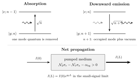
Mode-resolved absorption carries $n$, while downward emission carries the combined occupied-mode and vacuum factor $n+1$. At the ensemble level, stimulated emission amplifies a selected traveling mode only when its upper-state contribution exceeds absorption and all other propagation losses.

Three Complementary Descriptions

Stimulated emission appears in several formalisms. They answer different questions and should not be mixed without checking their assumptions.

Number-state description

The Fock-state transition

$$|e;n\rangle \longrightarrow |g;n+1\rangle$$

is best for:

• identifying the $n+1$ operator factor;
• separating vacuum and occupation-dependent contributions;
• counting photons in a specified mode;
• analyzing few-photon or cavity processes.

A number state has no definite optical phase. Therefore the statement “stimulated emission has the phase of the incident photon” is not meaningful for a pure Fock state.

Coherent-field description

A coherent state satisfies

$$a|\alpha\rangle = \alpha|\alpha\rangle, \qquad \overline n = |\alpha|^2.$$

For large $\overline n$, replacing the field operator by its coherent amplitude leads to a prescribed classical drive. The induced matter polarization can radiate phase coherently into that drive, increasing the field amplitude in a phase-matched mode.

The exact conditional field operation is still

$$a^\dagger|\alpha\rangle,$$

which is a photon-added coherent state and is not exactly proportional to $|\alpha\rangle$. The classical picture becomes accurate when one added quantum changes a highly occupied mode only by a small relative amount.

Incoherent-rate description

If field phase memory and optical coherence can be neglected, populations may obey Einstein or cross-section rate equations. This is appropriate for:

• broadband or incoherent radiation;
• weak probes in media with rapid dephasing;
• population kinetics averaged over many events;
• small-signal amplifier calculations.

It is not appropriate for a short coherent pulse that produces resolved Rabi oscillations. Coherent evolution may later reduce to a rate equation after adiabatic elimination of the optical coherence, but that reduction must be stated.

One process, different retained information

Description	Retains	Common output
Quantized mode	photon number and atom–field amplitudes	$n+1$, few-photon dynamics
Semiclassical coherent field	optical phase and matter coherence	Rabi frequency, susceptibility
Einstein kinetics	populations and spectral energy density	upward and downward rates
Propagation model	intensity, cross sections, spatial loss	gain per unit length

These descriptions agree in their common weak-coupling limits. They are not interchangeable outside those limits.

Relation to Einstein Coefficients

For lower and upper level populations $\mathcal N_1$ and $\mathcal N_2$ in an isotropic radiation field, the sharp-line Einstein model gives

$$\mathcal R_{\mathrm{abs}} = \mathcal N_1 B_{12}^{(\omega)} u_\omega(\omega_0),$$ $$\mathcal R_{\mathrm{stim}} = \mathcal N_2 B_{21}^{(\omega)} u_\omega(\omega_0),$$

and

$$\mathcal R_{\mathrm{sp}} = \mathcal N_2 A_{21}.$$

Here $u_\omega$ is total isotropic radiation energy density per unit angular frequency. The superscript is essential because changing the spectral variable changes the numerical $B$ coefficient.

The net stimulated production of radiation quanta is

$$\begin{aligned} \mathcal R_{\mathrm{net}} &= \mathcal R_{\mathrm{stim}} - \mathcal R_{\mathrm{abs}} \\ &= \left[ \mathcal N_2 B_{21}^{(\omega)} - \mathcal N_1 B_{12}^{(\omega)} \right] u_\omega. \end{aligned}$$

Thermal detailed balance gives

$$g_1B_{12}^{(\omega)} = g_2B_{21}^{(\omega)}.$$

Therefore,

$$\begin{aligned} \mathcal R_{\mathrm{net}} &= B_{21}^{(\omega)} u_\omega \\ &\quad\times \left( \mathcal N_2 - \frac{g_2}{g_1} \mathcal N_1 \right). \end{aligned}$$

Ordinary two-level gain requires

$$\frac{\mathcal N_2}{g_2} > \frac{\mathcal N_1}{g_1}.$$

This is population inversion per substate. The shortcut $\mathcal N_2>\mathcal N_1$ is valid only when $g_1=g_2$ and the two line profiles are reciprocal.

Thermal occupation check

For a thermal free-space field and matching Einstein conventions,

$$\frac{ \mathcal R_{\mathrm{stim}} }{ \mathcal R_{\mathrm{sp}} } = \frac{ B_{21}^{(\omega)}u_\omega }{ A_{21} } = \overline n(\omega_0,T),$$

where

$$\overline n(\omega,T) = \frac{1}{ e^{\hbar\omega/(k_{\mathrm B}T)}-1 }.$$

Thermal stimulation is consequently negligible for most optical transitions at room temperature but can dominate at microwave frequencies. Absorption from the same thermal field must be included at the same time.

From Event Rates to Cross Sections

Einstein coefficients are natural for isotropic radiation. A directed probe beam is usually described by cross sections.

For a monochromatic traveling wave with photon flux

$$\Phi = \frac{I}{\hbar\omega},$$

define the weak-field rates per particle by

$$W_{\mathrm{abs}} = \sigma_a(\omega)\Phi,$$ $$W_{\mathrm{stim}} = \sigma_e(\omega)\Phi.$$

Both $\sigma_a$ and $\sigma_e$ have dimensions of area. They include the declared polarization, line shape, and averaging over magnetic or molecular substates.

For resolved reciprocal substates,

$$\sigma_a(\omega) = \sigma_e(\omega)$$

when the same field mode and normalization are used. For level-averaged cross sections with reciprocal profiles,

$$g_1\sigma_a(\omega) = g_2\sigma_e(\omega).$$

Broad vibronic manifolds need more care: emission and absorption profiles can differ because the initial sublevel distributions differ. Relations such as the McCumber relation require thermalized manifolds and additional spectroscopic assumptions; they are not universal identities between arbitrary measured spectra.

Two-level weak-probe cross section

For a nondegenerate electric-dipole transition driven by a plane wave, define

$$\Omega = \frac{ \left| \boldsymbol\epsilon\mathbin{\cdot}\mathbf d_{eg} \right| E_0 }{ \hbar },$$

with

$$I = \frac12\epsilon_0cE_0^2.$$

If the optical coherence decays at rate $\gamma_2$, adiabatic elimination in the weak-field limit gives the stimulated rate coefficient

$$W(\Delta) = \frac{\Omega^2}{2} \frac{\gamma_2}{ \Delta^2+\gamma_2^2 }.$$

Dividing by photon flux yields

$$\begin{aligned} \sigma(\Delta) &= \frac{ \omega \left| \boldsymbol\epsilon\mathbin{\cdot}\mathbf d_{eg} \right|^2 }{ \epsilon_0c\hbar } \\ &\quad\times \frac{\gamma_2}{ \Delta^2+\gamma_2^2 }. \end{aligned}$$

This formula is state and polarization specific. For a closed, lifetime-limited, optimally polarized transition,

$$\gamma_2 = \frac{\Gamma}{2},$$

and the resonant value becomes

$$\sigma_0 = \frac{3\lambda_0^2}{2\pi}.$$

Branching, Clebsch–Gordan coefficients, polarization mismatch, pure dephasing, Doppler averaging, and inhomogeneous broadening reduce or redistribute the effective peak cross section. The compact resonant formula must not be applied to an arbitrary multilevel line without those factors.

Gain in a Traveling-Wave Medium

Consider a narrow probe propagating along $z$. In the weak-probe, slowly-varying limit,

$$\frac{dI(\omega,z)}{dz} = g_0(\omega)I(\omega,z),$$

where the small-signal net gain coefficient is

$$\begin{aligned} g_0(\omega) ={}& \mathcal N_2\sigma_e(\omega) - \mathcal N_1\sigma_a(\omega) \\ &- \alpha_{\mathrm{bg}}(\omega). \end{aligned}$$

Each term has dimensions of inverse length. The signs have direct meanings:

• $\mathcal N_2\sigma_e$ adds probe photons by stimulated emission;
• $\mathcal N_1\sigma_a$ removes probe photons by absorption;
• $\alpha_{\mathrm{bg}}$ includes scattering, parasitic absorption, and other distributed losses.

If the populations and cross sections are constant over a length $L$,

$$I(L) = I(0)e^{g_0L}.$$

The power gain is

$$G = \frac{I(L)}{I(0)} = e^{g_0L},$$

and its decibel value is

$$G_{\mathrm{dB}} = 10\log_{10}G.$$

A positive stimulated-emission term does not guarantee net amplification. The net coefficient must satisfy

$$g_0(\omega)>0.$$

Gain as negative absorption

With the propagation convention

$$\frac{dI}{dz} = -\alpha I,$$

an amplifying medium has

$$\alpha(\omega)<0, \qquad g(\omega)=-\alpha(\omega)>0.$$

In linear-response language, inversion reverses the sign of the dissipative part of the resonant susceptibility. This does not violate passivity because the pumped medium is not in thermal equilibrium: the amplified field draws energy from stored excitation supplied by the pump.

Gain bandwidth

The sign and size of $g_0$ depend on frequency through:

• homogeneous natural, collisional, and power-broadened profiles;
• Doppler or static inhomogeneous distributions;
• upper- and lower-manifold populations;
• polarization-dependent line strengths;
• reabsorption and background loss;
• the pump-induced spatial distribution of inversion.

An integrated line strength constrains area under a cross-section profile, whereas peak gain also depends on linewidth. Broadening can lower a peak without changing the relevant integrated strength.

Including spontaneous photons

Spontaneous emission into the observed spatial and spectral mode acts as a source term:

$$\frac{dI}{dz} = g_0I+j_{\mathrm{sp}}.$$

For constant $g_0\ne0$ and $j_{\mathrm{sp}}$,

$$\begin{aligned} I(L) ={}& I(0)e^{g_0L} \\ &+ \frac{j_{\mathrm{sp}}}{g_0} \left( e^{g_0L}-1 \right). \end{aligned}$$

The first term is amplified input. The second is amplified spontaneous emission. Its directional and spectral narrowing can resemble laser output, but it does not by itself establish resonator-defined oscillation or laser-like phase coherence.

Gain Saturation

Small-signal gain assumes that the probe does not appreciably change the populations. A strong field stimulates enough transitions to deplete the inversion, so the gain becomes intensity dependent.

A minimal homogeneous model

Take equal degeneracies and equal cross sections,

$$\sigma_a = \sigma_e = \sigma.$$

Let

$$D = \mathcal N_2-\mathcal N_1$$

be the inversion density. Suppose pumping and relaxation restore a no-probe inversion $D_0$ on a time scale $T_1$. A stimulated transition moves one particle from one level to the other, changing $D$ by two. With

$$W = \frac{\sigma I}{\hbar\omega},$$

the rate equation is

$$\frac{dD}{dt} = \frac{D_0-D}{T_1} - 2WD.$$

The steady inversion is

$$D_{\mathrm{ss}} = \frac{D_0}{ 1+I/I_{\mathrm{sat}} },$$

with

$$I_{\mathrm{sat}} = \frac{ \hbar\omega }{ 2\sigma T_1 }.$$

If

$$g_{\mathrm{gross},0} = \sigma D_0,$$

then

$$g_{\mathrm{net}}(I) = \frac{ g_{\mathrm{gross},0} }{ 1+I/I_{\mathrm{sat}} } - \alpha_{\mathrm{bg}}.$$

This is a model, not a universal law. The factor of two follows from a closed two-level inversion definition. A rapidly emptied lower laser level, multilevel branching, coherent saturation, pulsed extraction, spatial hole burning, or pump depletion changes the saturation scale and sometimes the functional form.

Homogeneous and inhomogeneous saturation

In a homogeneously broadened ensemble, all emitters within the line share the same transition frequency to the accuracy of the model. A strong narrow field can therefore reduce gain across the homogeneous profile.

In an inhomogeneously broadened ensemble, a narrow field first depletes the resonant subensemble. This can burn a spectral hole while off-resonant subensembles retain inversion. Collisions, spectral diffusion, and velocity changing processes can refill the hole.

Saturation is not damage

Gain saturation is reversible population redistribution caused by the signal. It should be distinguished from:

• irreversible photochemical or dielectric damage;
• thermal lensing;
• excited-state absorption;
• multiphoton ionization;
• pump depletion;
• nonlinear refractive effects.

Several can occur together in a real amplifier, but they have different scalings and recovery times.

How a Medium Acquires Gain

Pumping and relaxation pathways

An ordinary gain medium needs:

1. a pump that supplies free energy;
2. a pathway that populates the upper laser level;
3. sufficiently slow loss from that upper level;
4. sufficiently rapid removal from, or weak occupation of, the lower laser level;
5. a transition cross section large enough to overcome propagation losses.

The pump can be optical, electrical, chemical, collisional, or another nonequilibrium source. Stimulated emission transfers stored excitation to the signal; it does not supply the energy being amplified.

Why resonant two-level pumping does not create inversion

Let one incoherent resonant field drive both directions at rate $W$, and let the upper state decay at rate $\Gamma$. For a closed two-level system,

$$\frac{d\mathcal N_2}{dt} = W\mathcal N_1 - W\mathcal N_2 - \Gamma\mathcal N_2.$$

At steady state,

$$\frac{\mathcal N_2}{\mathcal N_1} = \frac{W}{W+\Gamma} < 1.$$

Increasing the resonant pump only approaches equal populations. It does not invert the same isolated transition. Three- and four-level schemes evade this ceiling by pumping through additional states and using asymmetric relaxation pathways.

The inversion criterion has a domain

Population inversion is required for gain in an ordinary reciprocal two-level medium whose response is described only by populations. It is not a theorem covering every driven multilevel quantum system.

Coherences can make distinct absorption amplitudes interfere destructively while leaving an emissive pathway. Such gain without inversion has been demonstrated in coherently driven multilevel atoms. This is a specialized interference effect, not evidence that the two-level balance condition was wrong.

Connection to Lasers

Stimulated emission is the microscopic amplification process in a conventional laser, but it is only one part of laser operation.

Amplifier, amplified spontaneous emission, and laser

• Traveling-wave amplifier: a pumped gain medium gives one-pass gain to an externally supplied signal without requiring feedback.
• Amplified spontaneous emission: spontaneous photons seed the pumped medium and are amplified without a required resonator or external input.
• Laser oscillator: feedback selects a self-consistent mode whose round-trip small-signal gain reaches threshold; no external seed is required.

A pumped single-pass medium can show stimulated emission and large gain without being a laser. Conversely, a resonator without net gain only stores and filters light; it does not sustain oscillation.

A simple round-trip threshold

Consider a uniform linear cavity of length $L$, mirror power reflectivities $R_1$ and $R_2$, gross material gain coefficient $g_{\mathrm m}$, and distributed internal loss $\alpha_{\mathrm i}$. One round trip multiplies the intracavity intensity by

$$\mathcal G_{\mathrm{rt}} = R_1R_2 \exp \left[ 2 \left( g_{\mathrm m}-\alpha_{\mathrm i} \right) L \right].$$

The small-signal threshold is

$$\mathcal G_{\mathrm{rt}} = 1,$$

or

$$\begin{aligned} g_{\mathrm{m,th}} ={}& \alpha_{\mathrm i} \\ &+ \frac{1}{2L} \ln \left( \frac{1}{R_1R_2} \right). \end{aligned}$$

Below threshold, a fluctuation decays after repeated round trips. Above threshold, it initially grows. In steady operation, saturation and pump depletion reduce the gain seen by the oscillating mode until round-trip gain balances round-trip loss.

This formula assumes uniform traveling-wave power gain on each pass and neglects standing-wave structure, spatial hole burning, mode competition, dispersion, and time dependence. Ring cavities and pulsed lasers require appropriately modified round-trip maps.

What sets the laser mode

Stimulated emission preferentially feeds whatever field modes are occupied, but occupation alone does not choose a unique mode. Selection also depends on:

• cavity resonances and diffraction loss;
• gain bandwidth and dispersion;
• spatial overlap with the pumped region;
• polarization-dependent gain and loss;
• nonlinear saturation and mode competition;
• spontaneous-emission noise and technical perturbations.

The coherent oscillator phase is a collective dynamical property of field, medium, feedback, and noise. It is not attached to an individual photon before the process.

Same Mode Does Not Mean Perfect Copy

The phrase “the emitted photon is identical to the stimulating photon” is a useful mode-label shorthand, but it can be misleading.

No individual photon is selected for copying

Photons in one mode are indistinguishable. The field changes from an $n$-excitation state to an $(n+1)$-excitation state; quantum mechanics does not label one photon as the original and another as its copy.

Creation is not a cloning map

For a coherent input,

$$a^\dagger|\alpha\rangle$$

is not the original coherent state with a separately cloned photon appended. Likewise, stimulated emission cannot clone an arbitrary unknown photonic quantum state.

A phase-preserving amplifier must add noise

An idealized single-mode phase-preserving power amplifier with gain $G$ can be represented as

$$a_{\mathrm{out}} = \sqrt G\,a_{\mathrm{in}} + e^{i\phi} \sqrt{G-1}\, b_{\mathrm{in}}^\dagger.$$

The auxiliary mode is necessary because

$$\begin{aligned} [a_{\mathrm{out}},a_{\mathrm{out}}^\dagger] &= G - (G-1) \\ &= 1. \end{aligned}$$

Without the second term, amplification would multiply the canonical commutator by $G$. Even when the auxiliary input is vacuum, its fluctuations appear as added amplifier noise. Spontaneous emission into the amplified mode is one physical manifestation of this unavoidable noise in an inverted-medium amplifier.

Experimental Signatures and Forward Models

Pump-on versus pump-off transmission

A weak probe can measure small-signal gain through

$$G(\omega) = \frac{ I_{\mathrm{out}}^{(\mathrm{pump\ on})} }{ I_{\mathrm{out}}^{(\mathrm{reference})} }.$$

The reference must be declared. Pump-off transmission may include ground-state absorption that disappears when the pump redistributes population. A measured increase can therefore contain both reduced absorption and true stimulated emission.

Seed dependence

In the linear regime,

$$I_{\mathrm{out}} \approx GI_{\mathrm{in}} + I_{\mathrm{ASE}}.$$

Varying $I_{\mathrm{in}}$ separates a seed-proportional term from the zero-seed intercept. At higher intensity, gain saturation bends the seed-proportional response.

Lifetime shortening under a resonant field

If lower-state reabsorption and repumping are negligible, an applied resonant mode adds a stimulated rate:

$$\Gamma_{\mathrm{obs}} = \Gamma_{\mathrm{tot}} + W_{\mathrm{stim}}.$$

An intensity-dependent lifetime can therefore measure a stimulated-emission cross section. In a dense or multilevel medium, radiation trapping, pump redistribution, cooperative emission, and excited-state absorption must be excluded before using this simple relation.

Direction and polarization

Stimulated output should appear in the phase-matched spatial and polarization mode of the seed, whereas uncollected free-space fluorescence occupies many modes. Finite numerical aperture, birefringence, recoil, collisions, and mode conversion blur this ideal distinction.

A Reliable Calculation Workflow

1. Declare the matter states. Include degeneracies, magnetic substates, vibrational manifolds, and relevant branching.
2. Declare the field mode. Specify frequency, polarization, direction, bandwidth, and spatial profile.
3. Choose the dynamical regime. Use coherent amplitudes, Einstein rates, or cross sections only after checking coherence and time scales.
4. Compute or obtain the line strength. Keep polarization and substate averaging explicit.
5. Build absorption and emission separately. Do not infer net gain from upper population alone.
6. Add all losses. Include lower-state reabsorption and background propagation loss.
7. Check the small-signal assumption. Compare the signal intensity with the appropriate saturation scale.
8. Propagate the observable. Solve for intensity or field amplitude with the correct spatial dependence.
9. Add spontaneous source noise when needed. It matters for ASE, threshold startup, linewidth, and quantum-limited amplification.
10. Test limiting cases. Recover absorption without inversion, transparency at balanced populations, exponential small-signal gain, and gain reduction under saturation.

Common Mistakes

Treating n + 1 as two unrelated mechanisms

Stimulated and spontaneous terms arise from one creation-operator matrix element. Their separation is useful in a weak-coupling rate description, but the underlying atom–field interaction is common.

Comparing one driven mode with all vacuum modes

The ratio $\Gamma_{\mathrm{stim}}/\Gamma_{\mathrm{sp}}=n$ applies to matched mode-resolved channels. Total free-space spontaneous emission sums over a continuum.

Assigning phase to a number state

A Fock state has definite occupation and undefined phase. Phase-coherent amplification belongs to a coherent-field or quadrature description.

Assuming an excited population implies gain

Absorption, degeneracies, spectral overlap, and background loss all enter. The condition is net:

$$\mathcal N_2\sigma_e - \mathcal N_1\sigma_a - \alpha_{\mathrm{bg}} > 0.$$

Using population inversion without degeneracies

For reciprocal level-averaged transitions, compare populations per substate, not just total populations.

Using a constant gain at arbitrary intensity

Exponential propagation with fixed $g_0$ is a small-signal result. A strong field depletes inversion and can also modify line shapes and the pump.

Calling every bright directional emission a laser

Amplified spontaneous emission can be bright, directional, and spectrally narrowed. Laser oscillation additionally requires a self-consistent feedback mode and round-trip gain–loss balance.

Saying stimulated emission creates free energy

The emitted photon energy comes from the excited medium. The pump supplied that stored energy, and the gain process depletes it.

Treating the resonant cross section as universal

The value $3\lambda^2/(2\pi)$ assumes a closed, optimally coupled, lifetime-limited two-level transition. Real lines carry branching, polarization, degeneracy, and broadening factors.

Key Results

1. Downward creation into a mode with occupation $n$ carries amplitude $\sqrt{n+1}$.
2. The $n$ term is stimulated emission; the unity is the vacuum contribution.
3. Absorption and stimulated emission have reciprocal microscopic strengths, so net gain depends on populations and degeneracies.
4. A directed weak probe sees $g_0=\mathcal N_2\sigma_e-\mathcal N_1\sigma_a-\alpha_{\mathrm{bg}}$.
5. Constant positive small-signal gain gives $I(L)=I(0)e^{g_0L}$.
6. Strong signals deplete inversion and saturate the gain.
7. A laser additionally needs pumping, feedback, mode selection, and round-trip gain equal to loss in steady operation.
8. Phase-preserving amplification necessarily adds quantum noise; stimulated emission is not a universal cloning operation.

Further Connections

• Einstein Coefficient Reference supplies the spectral-density Jacobians and degeneracy factors for stimulated $B$ coefficients.
• Linear Response Preview relates population contrast to the sign of resonant absorption.
• Line Shapes and Broadening explains how homogeneous and inhomogeneous widths redistribute peak cross section and gain.
• Optical Bloch Equations derive coherent saturation, scattering rates, and power broadening.
• Radiation Pressure tracks how absorption and stimulated emission transfer opposite momenta in a traveling mode.
• Einstein Coefficients gives the full $A/B$ convention ledger and degeneracy derivation.
• Spontaneous Emission develops the vacuum contribution, radiative lifetime, and emitted photon.
• Lasers and Quantum Technology places optical amplification in its experimental and historical setting.

References

1. A. Einstein, “Zur Quantentheorie der Strahlung,” Physikalische Zeitschrift 18, 121–128 (1917). The original introduction of the absorption, spontaneous-emission, and stimulated-emission coefficients.
2. P. A. M. Dirac, “The Quantum Theory of the Emission and Absorption of Radiation,” Proceedings of the Royal Society A 114, 243–265 (1927).
3. A. L. Schawlow and C. H. Townes, “Infrared and Optical Masers,” Physical Review 112, 1940–1949 (1958).
4. T. H. Maiman, “Stimulated Optical Radiation in Ruby,” Nature 187, 493–494 (1960).
5. D. E. McCumber, “Einstein Relations Connecting Broadband Emission and Absorption Spectra,” Physical Review 136, A954–A957 (1964).
6. C. M. Caves, “Quantum Limits on Noise in Linear Amplifiers,” Physical Review D 26, 1817–1839 (1982).
7. J. Kitching and L. Hollberg, “Interference-Induced Optical Gain Without Population Inversion in Cold, Trapped Atoms,” Physical Review A 59, 4685–4689 (1999).
8. C. Cohen-Tannoudji, J. Dupont-Roc, and G. Grynberg, Atom–Photon Interactions: Basic Processes and Applications (Wiley, 1992).
9. M. O. Scully and M. S. Zubairy, Quantum Optics (Cambridge University Press, 1997).
10. A. E. Siegman, Lasers (University Science Books, 1986).
11. R. Loudon, The Quantum Theory of Light, 3rd ed. (Oxford University Press, 2000).

Exercises

1. Occupation enhancement

Starting from the ladder-operator algebra, find the ratio of:

1. the total downward squared matrix element for $n=24$ to that for vacuum;
2. the stimulated part to the spontaneous part in the same mode;
3. the absorption squared matrix element to the total downward one at $n=24$.

Solution

The downward matrix element contains

$$\sqrt{n+1},$$

so its squared magnitude is proportional to $n+1$. Relative to vacuum,

$$\frac{n+1}{0+1} = 25.$$

The stimulated and spontaneous pieces are proportional to $n$ and $1$, respectively, so

$$\frac{ \Gamma_{\mathrm{stim}} }{ \Gamma_{\mathrm{sp}} } = n = 24.$$

Absorption is proportional to $n$, while total downward emission is proportional to $n+1$. Thus

$$\frac{ |M_{\mathrm{abs}}|^2 }{ |M_{\mathrm{down}}|^2 } = \frac{24}{25}.$$

These comparisons are for the same mode, matter matrix element, and line-broadening convention.

2. Thermal crossover

For a thermal mode, stimulated and spontaneous downward rates are equal when

$$\overline n(\omega,T)=1.$$

Derive the crossover temperature and evaluate it for:

1. $\nu=10.0\ \mathrm{GHz}$;
2. $\nu=500\ \mathrm{THz}$.

Solution

Set

$$\frac{1}{ e^{h\nu/(k_{\mathrm B}T)}-1 } = 1.$$

Then

$$e^{h\nu/(k_{\mathrm B}T)} = 2,$$

so

$$T_\times = \frac{ h\nu }{ k_{\mathrm B}\ln2 }.$$

For $10.0\ \mathrm{GHz}$,

$$\frac{h\nu}{k_{\mathrm B}} \simeq 0.480\ \mathrm K,$$

and therefore

$$T_\times \simeq 0.692\ \mathrm K.$$

For $500\ \mathrm{THz}$,

$$\frac{h\nu}{k_{\mathrm B}} \simeq 2.40\times10^4\ \mathrm K,$$

giving

$$T_\times \simeq 3.46\times10^4\ \mathrm K.$$

Thermal stimulation is therefore easy to encounter for microwave transitions and negligible for a visible-frequency transition at ordinary laboratory temperatures.

3. Degeneracy and inversion

A transition connects levels with

$$g_1=2, \qquad g_2=4.$$

The number densities are

$$\mathcal N_1 = 8.0\times10^{18}\ \mathrm{m^{-3}},$$ $$\mathcal N_2 = 1.2\times10^{19}\ \mathrm{m^{-3}}.$$

Assume reciprocal level-averaged line profiles and no background loss. Does the medium amplify even though $\mathcal N_2>\mathcal N_1$? Find the minimum upper-level density for gain.

Solution

The relevant populations are per substate:

$$\frac{\mathcal N_1}{g_1} = 4.0\times10^{18}\ \mathrm{m^{-3}},$$ $$\frac{\mathcal N_2}{g_2} = 3.0\times10^{18}\ \mathrm{m^{-3}}.$$

The upper population per substate is smaller, so absorption wins. The fact that the total upper population is larger is insufficient.

Threshold occurs at

$$\frac{\mathcal N_2}{g_2} = \frac{\mathcal N_1}{g_1}.$$

Therefore,

$$\mathcal N_{2,\mathrm{tr}} = \frac{g_2}{g_1} \mathcal N_1 = 1.6\times10^{19}\ \mathrm{m^{-3}}.$$

Strict gain requires a value above this transparency density.

4. Small-signal gain and decibels

At one frequency, a medium has

$$\begin{aligned} \mathcal N_2&=2.0\times10^{21}\ \mathrm{m^{-3}}, \\ \mathcal N_1&=4.0\times10^{20}\ \mathrm{m^{-3}}, \end{aligned}$$

with

$$\begin{aligned} \sigma_e&=2.0\times10^{-20}\ \mathrm{m^2}, \\ \sigma_a&=1.5\times10^{-20}\ \mathrm{m^2}, \end{aligned}$$

and

$$\alpha_{\mathrm{bg}} = 1.0\ \mathrm{m^{-1}}.$$

Find the net gain coefficient, the power gain through $L=5.0\ \mathrm{cm}$, and the gain in decibels.

Solution

The three propagation contributions are

$$\mathcal N_2\sigma_e = 40\ \mathrm{m^{-1}},$$ $$\mathcal N_1\sigma_a = 6.0\ \mathrm{m^{-1}},$$

and

$$\alpha_{\mathrm{bg}} = 1.0\ \mathrm{m^{-1}}.$$

Hence

$$g_0 = 40-6-1 = 33\ \mathrm{m^{-1}}.$$

The dimensionless gain exponent is

$$g_0L = 33(0.050) = 1.65.$$

Therefore,

$$G = e^{1.65} \simeq 5.21,$$

and

$$\begin{aligned} G_{\mathrm{dB}} &= 10\log_{10}(5.21) \\ &\simeq 7.17\ \mathrm{dB}. \end{aligned}$$

5. Derive homogeneous gain saturation

For the minimal inversion equation

$$\frac{dD}{dt} = \frac{D_0-D}{T_1} - 2 \frac{\sigma I}{\hbar\omega} D,$$

derive the steady inversion, identify the saturation intensity, and find the intensity at which the gross gain is one quarter of its small-signal value.

Solution

At steady state,

$$0 = \frac{D_0-D}{T_1} - 2 \frac{\sigma I}{\hbar\omega} D.$$

Multiplying by $T_1$ and collecting $D$ gives

$$D_0 = D \left( 1+ \frac{ 2\sigma T_1I }{ \hbar\omega } \right).$$

Define

$$I_{\mathrm{sat}} = \frac{ \hbar\omega }{ 2\sigma T_1 }.$$

Then

$$D = \frac{D_0}{ 1+I/I_{\mathrm{sat}} }.$$

Because gross gain is proportional to $D$,

$$\frac{ g_{\mathrm{gross}}(I) }{ g_{\mathrm{gross},0} } = \frac{1}{ 1+I/I_{\mathrm{sat}} }.$$

Setting this ratio to $1/4$ gives

$$1+\frac{I}{I_{\mathrm{sat}}} = 4,$$

so

$$I = 3I_{\mathrm{sat}}.$$

6. Cavity threshold

A linear cavity has

$$L=0.300\ \mathrm m,$$ $$R_1=0.990, \qquad R_2=0.900,$$

and

$$\alpha_{\mathrm i} = 0.050\ \mathrm{m^{-1}}.$$

Find the threshold gross material gain coefficient.

Solution

Use

$$g_{\mathrm{m,th}} = \alpha_{\mathrm i} + \frac{1}{2L} \ln \left( \frac{1}{R_1R_2} \right).$$

The mirror product is

$$R_1R_2 = 0.891.$$

Therefore,

$$\begin{aligned} g_{\mathrm{m,th}} &= 0.050 + \frac{1}{0.600} \ln \left( \frac{1}{0.891} \right) \\ &\simeq 0.242\ \mathrm{m^{-1}}. \end{aligned}$$

This is a power-gain coefficient. Using amplitude reflectivities without changing the exponent would introduce a factor-of-two error.

7. A photon-added coherent state

Normalize the photon-added coherent state

$$|\psi\rangle \propto a^\dagger|\alpha\rangle$$

and find its fidelity with $|\alpha\rangle$. Interpret the limits $|\alpha|\to0$ and $|\alpha|\to\infty$.

Solution

Its norm is

$$\begin{aligned} \langle\alpha| aa^\dagger |\alpha\rangle &= \langle\alpha| \left( a^\dagger a+1 \right) |\alpha\rangle \\ &= |\alpha|^2+1. \end{aligned}$$

Thus

$$|\psi\rangle = \frac{ a^\dagger|\alpha\rangle }{ \sqrt{|\alpha|^2+1} }.$$

The overlap is

$$\langle\alpha|\psi\rangle = \frac{\alpha^*}{ \sqrt{|\alpha|^2+1} },$$

so the fidelity is

$$F = \frac{|\alpha|^2}{ |\alpha|^2+1 }.$$

For $|\alpha|\to0$, the operation creates a one-photon state orthogonal to vacuum, so $F\to0$. For a highly occupied coherent mode, $F\to1$: one added quantum causes a small relative disturbance. It is still not an exact cloning operation at finite occupation.

8. Why an amplifier needs an auxiliary mode

Suppose one tries to amplify a bosonic mode by

$$a_{\mathrm{out}} = \sqrt G\,a_{\mathrm{in}}, \qquad G>1.$$

Show why this is not a valid canonical transformation. Then verify that

$$a_{\mathrm{out}} = \sqrt G\,a_{\mathrm{in}} + \sqrt{G-1}\, b_{\mathrm{in}}^\dagger$$

preserves the output commutator when $a$ and $b$ are independent bosonic modes.

Solution

The naive map gives

$$\begin{aligned} [a_{\mathrm{out}},a_{\mathrm{out}}^\dagger] &= G [a_{\mathrm{in}},a_{\mathrm{in}}^\dagger] \\ &= G, \end{aligned}$$

which is inconsistent with the required bosonic commutator $1$.

For the two-mode map, independence gives

$$[a_{\mathrm{in}},b_{\mathrm{in}}] = [a_{\mathrm{in}},b_{\mathrm{in}}^\dagger] = 0.$$

Therefore,

$$\begin{aligned} [a_{\mathrm{out}},a_{\mathrm{out}}^\dagger] &= G[a,a^\dagger] + (G-1)[b^\dagger,b] \\ &= G-(G-1) \\ &= 1. \end{aligned}$$

The auxiliary mode restores the commutator, but its fluctuations enter the output. This is the algebraic origin of the added-noise requirement for a phase-preserving amplifier.