Gauge Choices in Light–Matter Physics

Gauge freedom allows one electromagnetic situation to be represented by different potentials, canonical momenta, wavefunction phases, and light–matter interaction terms. In an exact calculation, properly related representations give the same predictions for physical observables. In a truncated calculation, they need not.

That last sentence explains both the usefulness and the danger of gauge choice in atomic, molecular, and optical physics. A convenient representation can expose the important scale or symmetry. An inconsistent combination of gauge choice, basis truncation, field-mode truncation, and observable can create a spurious physical disagreement.

The standard names require context:

• Coulomb gauge is a gauge condition on the vector potential.
• Velocity gauge usually means the minimal-coupling interaction written with a spatially uniform vector potential.
• Length gauge usually means the electric-dipole interaction $-\mathbf d\cdot\mathbf E$ obtained after a long-wavelength reduction and a time-dependent unitary transformation.
• Multipolar or dipole gauge usually refers to the Power–Zienau–Woolley representation of quantized matter and radiation, followed, when stated, by a multipole or electric-dipole approximation.

These labels overlap in common limits, but they are not universal synonyms.

Canonical Scope

This page owns the AMO comparison among common representations and the practical rules for translating between them. It does not rederive gauge redundancy from first principles. That material lives in Gauge Transformations in Quantum Mechanics and Gauge Transformations: First Encounter. The many-charge parent Hamiltonian and its $A^2$ term live in Minimal Coupling.

The purpose here is operational:

1. state which transformation or approximation produced a Hamiltonian;
2. know which state and observable belong to that representation;
3. understand why exact length and velocity forms agree;
4. recognize when finite bases, few-level models, or few-mode models destroy that agreement;
5. use disagreement as a convergence diagnostic rather than as evidence for different physics.

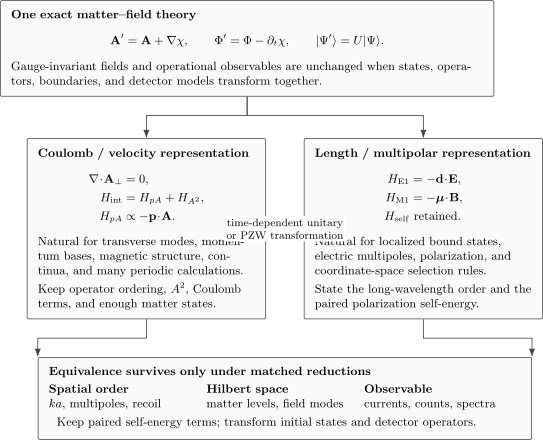
Gauge-related Hamiltonians are equivalent only as complete packages. The state, canonical operators, field variables, self-energy term, and detector observable must follow the same transformation. Spatial, level, and mode truncations are separate operations.

Gauge Transformations

For prescribed electromagnetic potentials, choose a real function $\chi(\mathbf r,t)$ and transform

$$\begin{aligned} \mathbf A' &= \mathbf A+\boldsymbol\nabla\chi, \\ \Phi' &= \Phi-\partial_t\chi. \end{aligned}$$

The fields are unchanged:

$$\mathbf B' = \boldsymbol\nabla\times\mathbf A' = \mathbf B,$$

and

$$\mathbf E' = - \boldsymbol\nabla\Phi' - \partial_t\mathbf A' = \mathbf E.$$

For particles with charges $q_a$, the matter state transforms with

$$U_\chi(t) = \exp \left[ \frac{i}{\hbar} \sum_a q_a\chi(\mathbf r_a,t) \right].$$

Thus

$$|\Psi'\rangle = U_\chi|\Psi\rangle.$$

The Hamiltonian is not transformed by similarity alone when $U_\chi$ depends on time:

$$H' = U_\chi H U_\chi^\dagger + i\hbar \left( \partial_tU_\chi \right) U_\chi^\dagger.$$

The additional term is essential. It produces the scalar-potential shift and ensures that

$$i\hbar\partial_t|\Psi'\rangle = H'|\Psi'\rangle.$$

States and observables transform together

For an observable $O$,

$$O' = U_\chi O U_\chi^\dagger.$$

Then

$$\langle\Psi'|O'|\Psi'\rangle = \langle\Psi|O|\Psi\rangle.$$

Comparing $\langle\Psi'|O|\Psi'\rangle$ with $\langle\Psi|O|\Psi\rangle$ while leaving $O$ untransformed is generally not a gauge-equivalence test.

The same rule applies to:

• projectors used to define populations;
• current and momentum operators;
• jump operators in master equations;
• input and output field operators;
• photodetection models;
• initial and final scattering states.

Three operations that should not be conflated

Operation	What it does	Does it change exact physics?
gauge fixing	selects a representative satisfying a condition such as $\boldsymbol\nabla\cdot\mathbf A=0$	no
unitary change of representation	redistributes canonical matter and field variables	no, when complete
approximation or projection	removes spatial orders, levels, modes, or reservoir memory	possibly

The difficulty is that a projection need not commute with a unitary transformation. “Choose a gauge” and “truncate to two levels” are not one operation.

Coulomb Gauge

Coulomb gauge imposes

$$\boldsymbol\nabla \mathbin{\cdot} \mathbf A_\perp = 0.$$

It separates the electric field into longitudinal and transverse parts:

$$\mathbf E = \mathbf E_\parallel + \mathbf E_\perp,$$

with

$$\mathbf E_\parallel = - \boldsymbol\nabla\Phi, \qquad \mathbf E_\perp = - \partial_t\mathbf A_\perp.$$

For charge density $\rho$ in free space, the scalar potential obeys

$$-\nabla^2\Phi = \frac{\rho}{\epsilon_0}$$

up to boundary conditions and external sources. The longitudinal field is therefore constrained by the instantaneous charge configuration in this representation, while $\mathbf A_\perp$ contains the transverse radiative degrees of freedom.

Coulomb-gauge Hamiltonian

For nonrelativistic charges and quantized transverse radiation,

$$\begin{aligned} H_{\mathrm C} ={}& \sum_a \frac{ \left[ \mathbf p_a - q_a\mathbf A_\perp(\mathbf r_a) \right]^2 }{2m_a} \\ &+ V_{\mathrm C} + H_{\mathrm{EM}} + H_{\mathrm{ext}}. \end{aligned}$$

$V_{\mathrm C}$ contains the longitudinal Coulomb interaction, while $H_{\mathrm{EM}}$ contains transverse field modes. Expanding the square gives

$$H_{\mathrm C} = H_0 + H_{pA} + H_{A^2}.$$

The linear term is

$$\begin{aligned} H_{pA} ={}& - \sum_a \frac{q_a}{2m_a} \\ &\times \left[ \mathbf p_a \mathbin{\cdot} \mathbf A_\perp(\mathbf r_a) + \mathbf A_\perp(\mathbf r_a) \mathbin{\cdot} \mathbf p_a \right], \end{aligned}$$

and the quadratic term is

$$H_{A^2} = \sum_a \frac{q_a^2}{2m_a} \mathbf A_\perp^2(\mathbf r_a).$$

The Coulomb-gauge representation is often called a minimal-coupling representation. In a long-wavelength classical drive, it is also the common starting point for what AMO calculations call the velocity gauge.

Why Coulomb gauge is useful

Coulomb gauge makes several structures explicit:

• transverse photons are separated from longitudinal Coulomb forces;
• canonical field quantization is direct in free space and cavities;
• magnetic couplings and spatial mode profiles remain visible;
• momentum-space and continuum calculations can be natural;
• translation symmetry is often easier to preserve than in a coordinate coupling.

Its costs are equally real:

• $p\cdot A$ matrix elements are sensitive to basis completeness;
• $A^2$ must be retained at the matched order;
• a few-level matter truncation can converge poorly in some regimes;
• the canonical matter–field partition can be misleading when coupling is ultrastrong.

Residual freedom

The condition $\boldsymbol\nabla\cdot\mathbf A=0$ does not always fix the gauge uniquely. Residual gauge functions satisfy

$$\nabla^2\chi=0$$

and must also respect boundary and asymptotic conditions. In bounded or multiply connected domains, these conditions are part of the physical problem.

Velocity Gauge

In AMO strong-field and spectroscopy calculations, velocity gauge usually refers to a spatially uniform vector potential $\mathbf A(t)$ with $\Phi=0$:

$$H_{\mathrm V}(t) = \frac{ \left[ \mathbf p-q\mathbf A(t) \right]^2 }{2m} + V(\mathbf r).$$

This form already assumes that the field variation over the matter system has been neglected. It is therefore more specific than Coulomb gauge.

Expanding,

$$\begin{aligned} H_{\mathrm V}(t) ={}& H_0 - \frac{q}{m} \mathbf A(t) \mathbin{\cdot} \mathbf p \\ &+ \frac{q^2\mathbf A^2(t)}{2m}, \end{aligned}$$

where

$$H_0 = \frac{\mathbf p^2}{2m} + V(\mathbf r).$$

Because $\mathbf A(t)$ is spatially uniform, it commutes with $\mathbf p$.

Removing a c-number A² term

For one particle in a prescribed, spatially uniform field,

$$C(t) = \frac{q^2\mathbf A^2(t)}{2m}$$

is proportional to the identity in the matter Hilbert space. Write

$$|\psi_{\mathrm V}(t)\rangle = \exp \left[ - \frac{i}{\hbar} \int_{t_0}^{t} C(t')\,dt' \right] |\widetilde\psi_{\mathrm V}(t)\rangle.$$

Then $\widetilde\psi_{\mathrm V}$ evolves with

$$\widetilde H_{\mathrm V} = H_0 - \frac{q}{m} \mathbf A(t) \mathbin{\cdot} \mathbf p.$$

This phase removal is valid because the field is prescribed, uniform, and the particle number is fixed. It does not justify deleting $A^2$ when:

• $\mathbf A$ varies over the matter coordinates;
• the field is quantized;
• particle-number or charge sectors are coherently mixed;
• the quadratic term changes mode dynamics or stability;
• a gauge-equivalent self-energy term is required elsewhere.

Why velocity gauge is useful

Velocity gauge can be effective when:

• momentum and continuum components dominate;
• a spatial grid or plane-wave basis handles derivatives accurately;
• periodicity makes the position operator awkward;
• the pulse is represented naturally by $\mathbf A(t)$;
• high-energy states are included sufficiently far into the continuum.

Its convergence can be demanding in a short bound-state basis because momentum matrix elements encode contributions from remote states through commutator and sum-rule identities.

Length Gauge

For a prescribed field in the long-wavelength approximation, let

$$\mathbf A(\mathbf r,t) \simeq \mathbf A(t), \qquad \Phi=0.$$

Choose the gauge function

$$\chi(\mathbf r,t) = - \mathbf r \mathbin{\cdot} \mathbf A(t).$$

Then

$$\mathbf A_{\mathrm L} = \mathbf A+\boldsymbol\nabla\chi = \mathbf 0,$$

and

$$\begin{aligned} \Phi_{\mathrm L} &= - \partial_t\chi \\ &= \mathbf r \mathbin{\cdot} \dot{\mathbf A}(t) \\ &= - \mathbf r \mathbin{\cdot} \mathbf E(t). \end{aligned}$$

The state transforms with the Göppert–Mayer unitary

$$U_{\mathrm{LV}}(t) = \exp \left[ - \frac{iq}{\hbar} \mathbf r \mathbin{\cdot} \mathbf A(t) \right].$$

Applying the full time-dependent Hamiltonian transformation gives

$$H_{\mathrm L}(t) = \frac{\mathbf p^2}{2m} + V(\mathbf r) - q\mathbf r \mathbin{\cdot} \mathbf E(t).$$

With electric dipole

$$\mathbf d=q\mathbf r,$$

the interaction is

$$H_{\mathrm{int}}^{\mathrm L} = - \mathbf d \mathbin{\cdot} \mathbf E(t).$$

The $A^2$ term did not vanish by neglect. It was carried through a unitary transformation into the phase and scalar-potential representation.

Many-particle length form

For charges $q_a$ in a uniform field,

$$\mathbf d = \sum_a q_a\mathbf r_a.$$

The leading length-form interaction is

$$H_{\mathrm{int}}^{\mathrm L} = - \mathbf d \mathbin{\cdot} \mathbf E(t).$$

If coordinates are measured from an origin $\mathbf R_0$, define

$$\mathbf d_{\mathbf R_0} = \sum_a q_a \left( \mathbf r_a-\mathbf R_0 \right).$$

Shifting the origin by $\mathbf a$ gives

$$\mathbf d_{\mathbf R_0+\mathbf a} = \mathbf d_{\mathbf R_0} - Q\mathbf a, \qquad Q=\sum_aq_a.$$

For a neutral system, the total dipole is origin independent. For a charged system, an origin shift changes the coupling by a center-of-charge term. That change must be treated with the center-of-mass dynamics and the corresponding gauge phase; it is not evidence that the electric field has changed.

Why length gauge is useful

Length gauge often works well for:

• bound states localized in coordinate space;
• electric-dipole selection rules;
• low-order multiphoton processes in a converged bound-state basis;
• real-space propagation with well-controlled absorbing boundaries;
• pulse descriptions specified directly by $\mathbf E(t)$.

The form also makes physical polarization intuitive. Its limitations include:

• the unbounded position operator in continuum calculations;
• origin and boundary subtleties for charged systems;
• difficulties with periodic boundary conditions;
• the need for higher multipoles when $ka$ is not small;
• possible poor convergence for a basis optimized for momentum or translational structure.

The transformation is not the approximation

The long-wavelength replacement

$$\mathbf A(\mathbf r,t) \longrightarrow \mathbf A(t)$$

is an approximation. Once that replacement has been made, the velocity-to-length transformation above is exact within the reduced model. Conflating the spatial approximation with the unitary transformation makes it difficult to identify which step failed.

Length and Velocity Matrix Elements

Let $|i\rangle$ and $|f\rangle$ be exact eigenstates of

$$H_0 = \frac{\mathbf p^2}{2m} + V(\mathbf r),$$

with

$$H_0|n\rangle=E_n|n\rangle.$$

The commutator is

$$[H_0,\mathbf r] = - \frac{i\hbar}{m}\mathbf p.$$

Taking a matrix element gives

$$\mathbf p_{fi} = im\omega_{fi}\mathbf r_{fi},$$

where

$$\omega_{fi} = \frac{E_f-E_i}{\hbar}.$$

For a complex field convention proportional to $e^{-i\omega t}$,

$$\mathbf E(\omega) = i\omega\mathbf A(\omega).$$

The resonant velocity-form matrix element is therefore

$$\begin{aligned} - \frac{q}{m} \mathbf A \mathbin{\cdot} \mathbf p_{fi} ={}& - iq\omega_{fi} \mathbf A \mathbin{\cdot} \mathbf r_{fi}, \end{aligned}$$

while the length-form matrix element is

$$- q\mathbf E \mathbin{\cdot} \mathbf r_{fi} = - iq\omega \mathbf A \mathbin{\cdot} \mathbf r_{fi}.$$

They agree on resonance, $\omega=\omega_{fi}$, with the stated phase convention. More general response functions agree only after all intermediate states, contact terms, denominators, and transformed observables are included consistently.

Length and velocity oscillator strengths

Exact eigenstates give equivalent length and velocity forms. For one Cartesian component,

$$\left| p_{fi} \right|^2 = m^2\omega_{fi}^2 \left| x_{fi} \right|^2.$$

An approximate calculation may violate this relation because:

• the states are not exact eigenstates of the same Hamiltonian;
• the basis omits important bound or continuum states;
• a nonlocal effective potential modifies the velocity operator;
• relativistic or pseudopotential corrections are incomplete;
• transition energies and matrix elements come from inconsistent models.

Length–velocity disagreement is therefore a convergence and consistency diagnostic. It does not establish that one exact gauge predicts a different experiment.

Nonlocal effective Hamiltonians

If $H_0$ contains a nonlocal potential $V_{\mathrm{nl}}$, then

$$[V_{\mathrm{nl}},\mathbf r] \ne 0$$

in general. The physical velocity operator is

$$\mathbf v = \frac{i}{\hbar} [H_0,\mathbf r],$$

not automatically $\mathbf p/m$. Using a bare momentum matrix element with a nonlocal pseudopotential can create an artificial discrepancy between length and velocity forms.

Dipole and Multipolar Gauge Overview

The multipolar representation is obtained by a Power–Zienau–Woolley transformation of the coupled matter–field theory. It reorganizes charge and current densities into polarization and magnetization fields.

In one common convention, the transformation has the schematic form

$$U_{\mathrm{PZW}} = \exp \left[ - \frac{i}{\hbar} \int d^3r\, \mathbf P(\mathbf r) \mathbin{\cdot} \mathbf A_\perp(\mathbf r) \right].$$

The sign and the precise transverse polarization depend on the declared canonical convention. The important point is that the transformation acts on matter and field variables together.

The multipolar interaction is organized schematically as

$$\begin{aligned} H_{\mathrm{int}}^{\mathrm M} ={}& - \int d^3r\, \mathbf P \mathbin{\cdot} \mathbf E_\perp \\ &- \int d^3r\, \mathbf M \mathbin{\cdot} \mathbf B + H_{\mathrm{self}} + \cdots. \end{aligned}$$

Depending on the canonical field variable, the transverse electric coupling may be written using the displacement field rather than $\mathbf E_\perp$. The polarization self-energy or contact term paired with that convention is part of the Hamiltonian.

After a controlled multipole expansion about a matter center $\mathbf R$, the leading electric term is

$$H_{\mathrm{E1}} = - \mathbf d \mathbin{\cdot} \mathbf E(\mathbf R).$$

Magnetic-dipole, electric-quadrupole, Röntgen, recoil, and higher terms follow at subsequent orders or from center-of-mass motion. The dedicated multipole treatment owns their systematic derivation.

Dipole gauge versus length gauge

In a prescribed, spatially uniform classical field, “dipole gauge” and “length gauge” often refer to the same practical Hamiltonian $-\mathbf d\cdot\mathbf E(t)$.

In a quantized multimode theory, the terms are less interchangeable:

• length gauge often names the Göppert–Mayer transformation after a long-wavelength approximation;
• multipolar gauge names a representation of the full coupled matter–field theory;
• electric-dipole approximation names the leading spatial order;
• a polarization self-energy remains paired with the multipolar representation.

The calculation should state which meaning is intended.

Where the quadratic physics goes

The Coulomb-gauge $A^2$ term and the multipolar polarization self-energy are not identical term by term, but they belong to unitary-related complete Hamiltonians. Deleting $A^2$ before transformation and deleting the self-energy after transformation are parallel consistency failures.

The issue is especially visible in cavity and ultrastrong-coupling models, where these terms affect stability, sum rules, mode renormalization, and the meaning of bare photon and matter excitations.

Why Equivalent Formulations Look Different

Gauge-related descriptions can disagree visually in almost every intermediate object while agreeing in observables.

Canonical variables change

In velocity gauge, the mechanical momentum is

$$\boldsymbol\pi_{\mathrm V} = \mathbf p-q\mathbf A(t).$$

With

$$U_{\mathrm{LV}} = \exp \left[ - \frac{iq}{\hbar} \mathbf r\mathbin{\cdot}\mathbf A(t) \right],$$

one finds

$$U_{\mathrm{LV}} \boldsymbol\pi_{\mathrm V} U_{\mathrm{LV}}^\dagger = \mathbf p.$$

The symbol $\mathbf p$ in length gauge represents the transformed mechanical momentum of the reduced model. Comparing the same written canonical operator in both gauges without this map is not a physical comparison.

Bare subsystems change

For quantized fields, a gauge transformation can mix canonical matter and field variables. Consequently:

• a “bare atom” basis can be gauge dependent;
• a canonical photon annihilation operator can transform;
• bare photon number need not be gauge invariant;
• matter–field entanglement assigned to a chosen tensor-product split can depend on representation.

Operational detector records, emitted fluxes, spectra, and total energies remain the appropriate comparison targets when the detector model is transformed consistently.

Initial conditions change

Suppose a pulse has

$$\mathbf A(t_0)\ne\mathbf 0.$$

Then the corresponding length- and velocity-gauge states at $t_0$ differ by

$$|\psi_{\mathrm L}(t_0)\rangle = U_{\mathrm{LV}}(t_0) |\psi_{\mathrm V}(t_0)\rangle.$$

Using the same coordinate-space function as the initial state in both gauges prepares different physical states unless $U_{\mathrm{LV}}(t_0)$ is the identity up to a global phase.

The same warning applies at the end of a pulse if $\mathbf A(t_f)\ne0$. Apparent final populations in bare states can differ until the states and projectors are mapped to the same representation.

Degeneracy labels can change

Even within one gauge condition, different vector potentials can emphasize different symmetries. Landau Gauge and Symmetric Gauge shows how a uniform magnetic field can be organized by guiding-center momentum or angular momentum. The energy subspace is the same, but a basis change inside a degenerate level can accompany the gauge phase.

Truncation and Gauge Equivalence

Let $P$ project onto a finite matter basis. Starting from exact Hamiltonians related by $H'=UHU^\dagger$ for a time-independent illustration, compare

$$PH'P = PUHU^\dagger P$$

with a transformation inside the truncated space. In general,

$$PUP$$

is not unitary on the range of $P$, so the two projected models are not guaranteed to be equivalent.

Finite-dimensional canonical algebra

No finite-dimensional matrices satisfy

$$[x,p] = i\hbar I$$

exactly. Taking the trace would give

$$\operatorname{tr}[x,p] = 0$$

but

$$\operatorname{tr}(i\hbar I) = i\hbar d \ne 0$$

for dimension $d>0$. Every finite-level truncation therefore modifies the canonical algebra that underlies gauge transformations and oscillator strength sum rules.

This does not make few-level models useless. It means their accuracy must be benchmarked against the observable and coupling regime for which they are used.

Oscillator-strength sum rule

For one particle with a local potential, the double commutator gives

$$[x,[H_0,x]] = \frac{\hbar^2}{m}.$$

In an eigenstate $|i\rangle$,

$$\sum_n \left( E_n-E_i \right) \left| \langle n|x|i\rangle \right|^2 = \frac{\hbar^2}{2m}.$$

The sum includes the complete discrete and continuum spectrum. A short basis cannot generally satisfy it. Missing strength can then appear as length–velocity disagreement, incorrect diamagnetic cancellation, or gauge sensitivity.

Few-level and few-mode models

Gauge sensitivity becomes more visible when:

• the light–matter coupling is a sizable fraction of bare frequencies;
• only two or a few matter levels are retained;
• only one or a few field modes are retained;
• counter-rotating and self-energy terms matter;
• the measured observable depends on the dressed ground state;
• loss and detector operators are added after the Hamiltonian truncation.

There is active technical literature on gauge-consistent truncation strategies. Different constructions can be optimized for different observables and regimes. The conservative practice is to state the construction, retain paired terms, transform observables, and demonstrate convergence rather than declaring one gauge universally superior.

Computational Pitfalls

Incomplete bases

A finite basis resolves only part of the unitary transformation. Test:

• energies and target matrix elements versus basis size;
• length and velocity forms of transition strengths;
• oscillator-strength sums;
• high-energy and continuum contributions;
• sensitivity to the spatial box and absorbing boundary.

Agreement between gauges is strong evidence of consistency, but accidental agreement at one parameter value is not a convergence proof.

Mixing approximate Hamiltonians

The identity

$$\mathbf p_{fi} = im\omega_{fi}\mathbf r_{fi}$$

assumes states and energies from the same $H_0$ and the correct velocity operator. Combining experimental transition energies with momentum matrix elements from one approximate Hamiltonian and position matrix elements from another can spoil the relation.

Nonlocal potentials and pseudopotentials

For a nonlocal $V_{\mathrm{nl}}$, replace the naive velocity by

$$\mathbf v = \frac{\mathbf p}{m} + \frac{i}{\hbar} [V_{\mathrm{nl}},\mathbf r].$$

Omitting the commutator term can make a velocity-gauge calculation look gauge dependent even when the underlying effective model can be coupled consistently.

Periodic systems

The position operator is not an ordinary bounded operator under periodic boundary conditions. A naive $-\mathbf E\cdot\mathbf r$ term can violate periodicity. Length-gauge formulations for crystals use Berry connections, covariant derivatives in crystal momentum, or equivalent polarization constructions. Velocity gauge preserves translation structure more directly, but requires enough bands to satisfy sum rules.

Spatial discretization

On a grid or lattice, ordinary finite differences may not preserve local gauge covariance. Gauge-covariant link variables attach a phase

$$U_{ij} = \exp \left[ - \frac{iq}{\hbar} \int_{\mathbf r_i}^{\mathbf r_j} \mathbf A \mathbin{\cdot} d\boldsymbol\ell \right]$$

to a discrete hop. This is the continuum origin of Peierls phases and avoids changing the physics when the grid is rephased locally.

Pulse conventions and endpoints

Since

$$\mathbf E(t) = - \dot{\mathbf A}(t),$$

an electric pulse determines $\mathbf A(t)$ only up to a constant. State:

• the integration constant;
• whether $\mathbf A$ vanishes before and after the pulse;
• how initial and final states are transformed;
• whether a nonzero pulse area implies a residual vector potential.

Changing the constant in $\mathbf A$ without changing the state phase is not an innocuous numerical adjustment.

Open-system terms

If

$$\dot\rho = - \frac{i}{\hbar} [H,\rho] + \sum_j \mathcal D[L_j]\rho,$$

then a unitary change of representation requires

$$\rho' = U\rho U^\dagger, \qquad L_j' = UL_jU^\dagger,$$

together with the time-dependent Hamiltonian term. Transforming $H$ while leaving phenomenological jump or detector operators fixed can produce gauge-dependent decay and counting predictions.

Mixing interaction forms

Do not add

$$- \frac{q}{m} \mathbf A\mathbin{\cdot}\mathbf p$$

and

$$- \mathbf d\mathbin{\cdot}\mathbf E$$

as independent couplings for the same field and transition unless a carefully derived hybrid representation says to do so. They are usually alternative descriptions of the same leading interaction, not two physical mechanisms to sum.

Worked Examples

Velocity-to-length transformation for a pulse

Start with

$$H_{\mathrm V} = \frac{ \left[ \mathbf p-q\mathbf A(t) \right]^2 }{2m} + V(\mathbf r)$$

and

$$U(t) = \exp \left[ - \frac{iq}{\hbar} \mathbf r \mathbin{\cdot} \mathbf A(t) \right].$$

The canonical momentum transforms as

$$U\mathbf pU^\dagger = \mathbf p+q\mathbf A(t).$$

Therefore

$$U \left[ \mathbf p-q\mathbf A(t) \right] U^\dagger = \mathbf p.$$

The similarity-transformed kinetic energy is free of $\mathbf A$, but the time derivative contributes

$$\begin{aligned} i\hbar \left( \partial_tU \right) U^\dagger &= q\mathbf r \mathbin{\cdot} \dot{\mathbf A}(t) \\ &= - q\mathbf r \mathbin{\cdot} \mathbf E(t). \end{aligned}$$

Hence

$$H_{\mathrm L} = \frac{\mathbf p^2}{2m} + V(\mathbf r) - q\mathbf r \mathbin{\cdot} \mathbf E(t).$$

Dropping the $i\hbar\dot U U^\dagger$ term would miss the entire length-gauge interaction.

A transition-matrix check

Suppose

$$E_f-E_i = \hbar\omega_{fi}.$$

For polarization $\boldsymbol\epsilon$,

$$\langle f| \boldsymbol\epsilon \mathbin{\cdot} \mathbf p |i\rangle = im\omega_{fi} \langle f| \boldsymbol\epsilon \mathbin{\cdot} \mathbf r |i\rangle.$$

If a numerical calculation gives length matrix element $r_{fi}$ and velocity matrix element $p_{fi}$, define

$$\eta_{\mathrm{LV}} = \frac{ \left| p_{fi} \right| }{ m|\omega_{fi}| \left| r_{fi} \right| }.$$

An exact nonzero transition gives $\eta_{\mathrm{LV}}=1$. Deviation measures a consistency error, although it does not identify by itself whether the basis, Hamiltonian, velocity operator, or transition energy is responsible.

Why a magnetic field cannot be transformed away

If one could choose $\mathbf A'=0$ throughout a simply connected region, then

$$\mathbf B' = \boldsymbol\nabla\times\mathbf A' = \mathbf 0.$$

Gauge transformations preserve $\mathbf B$, so this is impossible wherever the physical magnetic field is nonzero. The length-gauge construction that sets a spatially uniform laser $\mathbf A(t)$ to zero relies on

$$\boldsymbol\nabla\times\mathbf A(t) = \mathbf 0$$

inside the long-wavelength reduced model. It cannot remove a genuine static magnetic field.

Two-level projection as a noncommuting operation

Let

$$P = |g\rangle\langle g| + |e\rangle\langle e|.$$

A gauge transformation $U$ generally connects $|g\rangle$ and $|e\rangle$ to components outside this subspace:

$$(I-P)U|g\rangle \ne 0.$$

Then

$$(PUP)^\dagger(PUP) \ne P$$

in general. The projected transformation is not unitary, so independently projected Coulomb- and dipole-representation Hamiltonians can differ. Adding more levels or constructing a gauge-consistent effective transformation is the remedy; declaring the discrepancy physical is not.

A Gauge-Choice Workflow

Choose a representation by observable and numerical structure, then verify it:

1. Start from the field geometry. Is the field prescribed or quantized, transverse or longitudinal, uniform or spatially structured?
2. State the parent Hamiltonian. Record Coulomb, self-energy, spin, center-of-mass, and field terms.
3. Separate transformations from approximations. List long-wavelength, multipole, level, mode, rotating-wave, and reservoir reductions in order.
4. Match the basis. Coordinate-localized bound states often favor length form; momentum, continuum, and periodic structure may favor velocity or Coulomb form.
5. Transform states and observables. Include projectors, currents, detector operators, and initial conditions.
6. Retain paired quadratic terms. Keep $A^2$ or the corresponding polarization self-energy at the required order.
7. Converge the calculation. Increase matter levels, field modes, box size, angular channels, and bandwidth.
8. Cross-check a second representation. Compare gauge-invariant observables, not bare canonical labels.

No gauge choice compensates for an uncontrolled physical approximation.

Common Mistakes

• Calling Coulomb, velocity, length, and dipole gauge exact synonyms.
• Changing potentials without transforming the state phase.
• Applying $H'=UHU^\dagger$ for a time-dependent $U$ and forgetting $i\hbar\dot U U^\dagger$.
• Treating the dipole approximation as part of gauge redundancy.
• Dropping $A^2$ in Coulomb gauge and the polarization self-energy in multipolar gauge.
• Comparing canonical momentum, bare photon number, or bare atomic population without transforming the observable.
• Using the same initial coordinate-space function in two gauges when $U(t_0)\ne I$.
• Interpreting length–velocity disagreement as two exact theories making different predictions.
• Using $\mathbf p/m$ as the velocity with a nonlocal pseudopotential.
• Using $-\mathbf E\cdot\mathbf r$ naively under periodic boundary conditions.
• Setting $\mathbf A=0$ in a region with nonzero magnetic field.
• Adding $p\cdot A$ and $-\mathbf d\cdot\mathbf E$ for the same retained field without deriving the combination.
• Transforming a Hamiltonian but leaving dissipators or detector operators fixed.
• Assuming a two-level projection preserves the canonical commutator or a full oscillator-strength sum rule.

Exercises

1. Derive the length-gauge potentials

Starting from $\Phi=0$ and spatially uniform $\mathbf A(t)$, use

$$\chi(\mathbf r,t) = - \mathbf r\mathbin{\cdot}\mathbf A(t)$$

to find $\mathbf A'$ and $\Phi'$.

Solution

The transformed vector potential is

$$\begin{aligned} \mathbf A' &= \mathbf A(t) + \boldsymbol\nabla \left[ - \mathbf r \mathbin{\cdot} \mathbf A(t) \right] \\ &= \mathbf A(t)-\mathbf A(t) \\ &= \mathbf 0. \end{aligned}$$

The scalar potential is

$$\begin{aligned} \Phi' &= - \partial_t\chi \\ &= \mathbf r \mathbin{\cdot} \dot{\mathbf A}(t) \\ &= - \mathbf r \mathbin{\cdot} \mathbf E(t), \end{aligned}$$

because $\mathbf E=-\dot{\mathbf A}$ in the starting representation. The potential-energy term is therefore

$$q\Phi' = - q\mathbf r \mathbin{\cdot} \mathbf E(t) = - \mathbf d \mathbin{\cdot} \mathbf E(t).$$

2. Remove a uniform classical A² phase

Let

$$H(t) = \widetilde H(t)+C(t)I.$$

Show that a time-dependent global phase removes $C(t)$ from the evolution. Why does the argument fail for a quantized-mode $A^2$ operator?

Solution

Write

$$|\psi(t)\rangle = e^{-i\theta(t)} |\widetilde\psi(t)\rangle,$$

with

$$\theta(t) = \frac{1}{\hbar} \int_{t_0}^{t} C(t')\,dt'.$$

Then

$$\begin{aligned} i\hbar\partial_t|\psi\rangle ={}& C(t)|\psi\rangle \\ &+ e^{-i\theta(t)} i\hbar \partial_t|\widetilde\psi\rangle. \end{aligned}$$

The equation $i\hbar\partial_t|\psi\rangle=H|\psi\rangle$ reduces to

$$i\hbar \partial_t|\widetilde\psi\rangle = \widetilde H |\widetilde\psi\rangle.$$

For a quantized mode,

$$A^2 \propto \left( a+a^\dagger \right)^2$$

is not proportional to the identity. It changes mode energies and can connect photon-number states, so no matter-only global phase removes it.

3. Length–velocity matrix relation

For a local potential, derive

$$\mathbf p_{fi} = im\omega_{fi}\mathbf r_{fi}.$$

Solution

Since

$$H_0 = \frac{\mathbf p^2}{2m} + V(\mathbf r),$$

and $[V,\mathbf r]=0$,

$$[H_0,\mathbf r] = - \frac{i\hbar}{m}\mathbf p.$$

Between eigenstates,

$$\begin{aligned} \langle f| [H_0,\mathbf r] |i\rangle &= \left( E_f-E_i \right) \mathbf r_{fi} \\ &= \hbar\omega_{fi} \mathbf r_{fi}. \end{aligned}$$

Equating the two forms gives

$$\hbar\omega_{fi} \mathbf r_{fi} = - \frac{i\hbar}{m} \mathbf p_{fi},$$

so

$$\mathbf p_{fi} = im\omega_{fi}\mathbf r_{fi}.$$

4. Thomas–Reiche–Kuhn sum rule

For one Cartesian coordinate and a local potential, derive

$$\sum_n \left( E_n-E_i \right) \left| x_{ni} \right|^2 = \frac{\hbar^2}{2m}.$$

Solution

First,

$$[H_0,x] = - \frac{i\hbar}{m}p_x.$$

Therefore

$$[x,[H_0,x]] = \frac{\hbar^2}{m}.$$

Insert completeness between the operators:

$$\begin{aligned} \langle i| [x,[H_0,x]] |i\rangle ={}& 2 \sum_n \left( E_n-E_i \right) \\ &\times \left| \langle n|x|i\rangle \right|^2. \end{aligned}$$

Equating this with $\hbar^2/m$ yields

$$\sum_n \left( E_n-E_i \right) \left| x_{ni} \right|^2 = \frac{\hbar^2}{2m}.$$

The complete sum includes continuum states. A finite discrete basis generally leaves a deficit.

5. Finite-dimensional obstruction

Prove that no pair of finite-dimensional matrices can satisfy $[x,p]=i\hbar I$.

Solution

For finite matrices, cyclicity of the trace gives

$$\operatorname{tr}[x,p] = \operatorname{tr}(xp) - \operatorname{tr}(px) = 0.$$

If the canonical commutator held in dimension $d$, then

$$\operatorname{tr}[x,p] = \operatorname{tr}(i\hbar I) = i\hbar d.$$

For $d>0$, this is nonzero, a contradiction. A finite-level model must modify the canonical algebra and cannot implement every exact gauge transformation internally.

6. Magnetic field cannot be gauged away

Show that no gauge transformation can set $\mathbf A'=0$ throughout a region where $\mathbf B\ne0$.

Solution

A gauge transformation preserves

$$\mathbf B = \boldsymbol\nabla\times\mathbf A.$$

If $\mathbf A'=0$ throughout the region, then

$$\mathbf B' = \boldsymbol\nabla\times\mathbf A' = 0.$$

But gauge invariance requires $\mathbf B'=\mathbf B$. Therefore $\mathbf A'=0$ is impossible wherever the physical magnetic field is nonzero.

The length-gauge construction can set a spatially uniform time-dependent $\mathbf A(t)$ to zero because that reduced vector potential has zero curl.

7. Coordinate shift versus gauge transformation

A neutral atom is redescribed using an internal coordinate origin shifted by $\mathbf a$. Is this relabeling by itself an electromagnetic gauge transformation? State what changes and what does not.

Solution

It is a coordinate or expansion-point change, not by itself an electromagnetic gauge transformation. A gauge transformation changes the potentials and the phase representation while leaving $\mathbf E$ and $\mathbf B$ invariant. A rigid shift instead changes the internal coordinate labels and redistributes higher multipole coefficients and plane-wave phases.

For a neutral system, the electric dipole operator is unchanged by the shift. For a charged system, permanent moments and monopole coupling must be transformed together. The full derivation, including off-diagonal transition dipoles, is at Dipole Approximation.

8. Pulse endpoint states

A velocity-gauge pulse has $\mathbf A(t_0)=\mathbf A_0\ne0$. If the physical initial state is the field-free eigenstate $|i\rangle$ in length gauge, what velocity-gauge state represents the same preparation?

Solution

The length- and velocity-gauge states obey

$$|\psi_{\mathrm L}(t)\rangle = U_{\mathrm{LV}}(t) |\psi_{\mathrm V}(t)\rangle,$$

where

$$U_{\mathrm{LV}}(t) = \exp \left[ - \frac{iq}{\hbar} \mathbf r \mathbin{\cdot} \mathbf A(t) \right].$$

Therefore

$$|\psi_{\mathrm V}(t_0)\rangle = U_{\mathrm{LV}}^\dagger(t_0) |i\rangle.$$

Explicitly,

$$|\psi_{\mathrm V}(t_0)\rangle = \exp \left[ \frac{iq}{\hbar} \mathbf r \mathbin{\cdot} \mathbf A_0 \right] |i\rangle.$$

Using the same unphased coordinate-space eigenfunction in both gauges would represent different canonical states when $\mathbf A_0\ne0$.

Further Connections

• Minimal Coupling owns the many-particle $p\cdot A$, $A^2$, scalar-potential, and field-mode ledger.
• Gauge Transformations in Quantum Mechanics owns gauge-equivalent states, operators, currents, and loop phases.
• Landau Gauge and Symmetric Gauge compares two useful representatives for a uniform magnetic field.
• Dipole Approximation owns the spatial long-wavelength expansion, transition dipoles, and expansion-point bookkeeping used after a representation is chosen.
• Multipole Operators develops the tensor structure used after a multipolar expansion.
• Transition Rates in Light–Matter Interaction connects consistently chosen interaction matrix elements to measured rates.
• Light–Matter Models provides compact few-level and few-mode Hamiltonian cards.

References

• C. Cohen-Tannoudji, J. Dupont-Roc, and G. Grynberg, Photons and Atoms: Introduction to Quantum Electrodynamics, Wiley, 1989.
• D. P. Craig and T. Thirunamachandran, Molecular Quantum Electrodynamics, Dover, 1998.
• M. Göppert-Mayer, “Über Elementarakte mit zwei Quantensprüngen,” Annalen der Physik 401, 273–294 (1931), doi:10.1002/andp.19314010303.
• E. A. Power and S. Zienau, “Coulomb gauge in non-relativistic quantum electro-dynamics and the shape of spectral lines,” Philosophical Transactions of the Royal Society A 251, 427–454 (1959), doi:10.1098/rsta.1959.0008.
• R. G. Woolley, “Gauge invariant wave mechanics and the Power–Zienau–Woolley transformation,” Journal of Physics A 13, 2795–2803 (1980), doi:10.1088/0305-4470/13/8/027.
• M. Babiker and R. Loudon, “Derivation of the Power–Zienau–Woolley Hamiltonian in quantum electrodynamics by gauge transformation,” Proceedings of the Royal Society A 385, 439–460 (1983), doi:10.1098/rspa.1983.0022.
• A. F. Starace, “Length and velocity formulas in approximate oscillator-strength calculations,” Physical Review A 3, 1242–1245 (1971), doi:10.1103/PhysRevA.3.1242.
• D. H. Kobe, “Gauge-invariant resolution of the controversy over length versus velocity forms of the interaction with electric dipole radiation,” Physical Review A 19, 205–214 (1979), doi:10.1103/PhysRevA.19.205.
• W. E. Lamb, R. R. Schlicher, and M. O. Scully, “Matter-field interaction in atomic physics and quantum optics,” Physical Review A 36, 2763–2772 (1987), doi:10.1103/PhysRevA.36.2763.
• A. Stokes and A. Nazir, “Gauge ambiguities imply Jaynes–Cummings physics remains valid in ultrastrong coupling QED,” Nature Communications 10, 499 (2019), doi:10.1038/s41467-018-08101-0.
• O. Di Stefano et al., “Resolution of gauge ambiguities in ultrastrong-coupling cavity quantum electrodynamics,” Nature Physics 15, 803–808 (2019), doi:10.1038/s41567-019-0534-4.
• A. Vukics, G. Kónya, and P. Domokos, “The gauge-invariant Lagrangian, the Power–Zienau–Woolley picture, and the choices of field momenta in nonrelativistic quantum electrodynamics,” Scientific Reports 11, 16337 (2021), doi:10.1038/s41598-021-94405-z.
• C. Gustin, S. Franke, and S. Hughes, “Gauge-invariant theory of truncated quantum light–matter interactions in arbitrary media,” Physical Review A 107, 013722 (2023), doi:10.1103/PhysRevA.107.013722.
• L. Yue and M. B. Gaarde, “Structure gauges and laser gauges for the semiconductor Bloch equations in high-order harmonic generation,” Physical Review A 101, 053411 (2020), doi:10.1103/PhysRevA.101.053411.