Gauge Transformations: First Encounter

Gauge transformations are changes of electromagnetic potentials that leave the electric and magnetic fields unchanged. In wave mechanics they also change the local phase convention of a charged-particle wavefunction. The physical state is not changed; the description is.

This page is a first encounter inside nonrelativistic wave mechanics. The broader structural meaning of gauge redundancy belongs to symmetry, geometry, and quantum field theory. Here the goal is practical: know how $\mathbf A$, $\Phi$, and $\psi$ transform, and know which quantities are safe to call physical.

Potentials Are Not Unique

The electromagnetic fields are

$$\mathbf E = - \nabla\Phi - \frac{\partial\mathbf A}{\partial t}, \qquad \mathbf B = \nabla\times\mathbf A.$$

A gauge transformation is specified by a real scalar function $\chi(\mathbf r,t)$:

$$\mathbf A' = \mathbf A+\nabla\chi, \qquad \Phi' = \Phi-\frac{\partial\chi}{\partial t}.$$

These new potentials describe the same fields. For the magnetic field,

$$\mathbf B' = \nabla\times\mathbf A' = \nabla\times\mathbf A + \nabla\times\nabla\chi = \mathbf B,$$

because the curl of a gradient vanishes. For the electric field,

$$\begin{aligned} \mathbf E' &= - \nabla\left( \Phi-\frac{\partial\chi}{\partial t} \right) - \frac{\partial}{\partial t} \left( \mathbf A+\nabla\chi \right) \\ &= - \nabla\Phi - \frac{\partial\mathbf A}{\partial t} = \mathbf E. \end{aligned}$$

Thus a gauge transformation changes the representative potentials, not the electromagnetic fields.

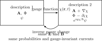
A gauge transformation gives a different potential pair and a different local phase convention for the wavefunction. Gauge-invariant fields, probabilities, and currents describe the same physics.

Why the Wavefunction Must Transform

For a particle of charge $q$, minimal coupling uses

$$\hat{\boldsymbol\pi} = - i\hbar\nabla - q\mathbf A.$$

This kinetic momentum appears in the Hamiltonian

$$\hat H = \frac{\hat{\boldsymbol\pi}^{\,2}}{2m} + q\Phi.$$

If $\mathbf A$ changes by $\nabla\chi$, the wavefunction must change by a compensating local phase:

$$\psi' = \exp\left( \frac{iq\chi}{\hbar} \right)\psi.$$

This is not an optional convention. Without this phase change, the minimally coupled Schrödinger equation would not keep the same form under a gauge transformation.

Covariant Momentum

The key identity is

$$\left( -i\hbar\nabla-q\mathbf A' \right)\psi' = \exp\left( \frac{iq\chi}{\hbar} \right) \left( -i\hbar\nabla-q\mathbf A \right)\psi.$$

In words: the kinetic momentum acting on the transformed wavefunction gives the transformed version of the old kinetic momentum acting on the old wavefunction.

This is why $\hat{\boldsymbol\pi}=-i\hbar\nabla-q\mathbf A$ is called gauge-covariant. The canonical momentum $-i\hbar\nabla$ alone is not gauge-covariant.

The time-dependent part transforms similarly:

$$\left( i\hbar\frac{\partial}{\partial t} - q\Phi' \right)\psi' = \exp\left( \frac{iq\chi}{\hbar} \right) \left( i\hbar\frac{\partial}{\partial t} - q\Phi \right)\psi.$$

Together these identities make the Schrödinger equation gauge-covariant.

What Stays Invariant

The probability density is unchanged:

$$\rho' = \lvert\psi'\rvert^2 = \lvert\psi\rvert^2 = \rho.$$

The gauge-covariant current

$$\mathbf j = \frac{1}{m} \operatorname{Re} \left[ \psi^* \left( -i\hbar\nabla-q\mathbf A \right)\psi \right]$$

is also unchanged when both $\mathbf A$ and $\psi$ are transformed. The local phase changes, but the vector potential changes at the same time, so the physical current agrees.

For a polar form

$$\psi = R e^{iS/\hbar},$$

the phase changes as

$$S'=S+q\chi.$$

The gauge-invariant velocity field depends on the combination

$$\nabla S-q\mathbf A,$$

not on $\nabla S$ alone.

Gauge Choice Versus Gauge Transformation

A gauge transformation maps one description to another equivalent description. A gauge choice is a decision to work in one representative.

Common examples include:

• Coulomb gauge, $\nabla\cdot\mathbf A=0$;
• temporal gauge, $\Phi=0$, when it can be imposed consistently;
• Landau gauge for a uniform magnetic field;
• symmetric gauge for a uniform magnetic field.

Choosing a gauge can make a calculation easier, but it should not change gauge-invariant predictions. If a computed energy, probability, or physical current depends on a gauge choice, something has been compared incorrectly or an incomplete set of states has been used.

Landau and Symmetric Gauge Example

For a uniform magnetic field

$$\mathbf B = B\hat{\mathbf z},$$

two useful vector potentials are the Landau gauge

$$\mathbf A_L = Bx\,\hat{\mathbf y}$$

and the symmetric gauge

$$\mathbf A_S = \frac{B}{2} \left( -y\,\hat{\mathbf x} + x\,\hat{\mathbf y} \right).$$

They differ by a gradient:

$$\mathbf A_L-\mathbf A_S = \frac{B}{2} \left( y\,\hat{\mathbf x} + x\,\hat{\mathbf y} \right) = \nabla\left( \frac{Bxy}{2} \right).$$

Thus the gauge function connecting symmetric gauge to Landau gauge is

$$\chi = \frac{Bxy}{2}.$$

If $\psi_S$ is a wavefunction in symmetric gauge, the corresponding Landau-gauge representative is

$$\psi_L = \exp\left( \frac{iqBxy}{2\hbar} \right)\psi_S.$$

The wavefunction formulas look different, and the convenient labels are different, but the magnetic field and energy spectrum are the same.

Local Phases and Global Effects

If $\chi$ is constant, the gauge transformation is just a global phase:

$$\psi' = e^{iq\chi/\hbar}\psi.$$

If $\chi$ depends on position and time, the phase is local. Local phase changes are not directly observable by themselves, but gauge-invariant phase differences around closed loops can matter. The Aharonov–Bohm effect is the standard example: a region with $\mathbf B=0$ along the particle path can still have physically meaningful magnetic flux through an excluded region.

The lesson is not that the vector potential is itself directly observable in a gauge-dependent way. The lesson is that quantum phases, potentials, and topology must be combined into gauge-invariant quantities.

Common Mistakes

• Changing $\mathbf A$ and $\Phi$ without changing the wavefunction phase.
• Treating the canonical momentum $-i\hbar\nabla$ as the mechanical momentum in a vector potential.
• Saying the vector potential is “unphysical” and then ignoring its role in the wave equation.
• Comparing wavefunctions written in different gauges as if they were the same representative.
• Expecting gauge-dependent labels, such as a particular conserved canonical momentum in a chosen gauge, to be universal observables.
• Confusing gauge redundancy with an ordinary physical symmetry that maps one physical state to a different physical state.

Exercises

1. Verify that the gauge transformation leaves $\mathbf B$ unchanged.

Solution

Using

$$\mathbf A' = \mathbf A+\nabla\chi,$$

we find

$$\mathbf B' = \nabla\times\mathbf A' = \nabla\times\mathbf A + \nabla\times\nabla\chi.$$

Since $\nabla\times\nabla\chi=0$,

$$\mathbf B'=\mathbf B.$$

2. Show that the probability density is gauge invariant.

Solution

The transformed wavefunction is

$$\psi' = e^{iq\chi/\hbar}\psi.$$

Since the phase has unit magnitude,

$$\lvert\psi'\rvert^2 = \left\lvert e^{iq\chi/\hbar}\right\rvert^2 \lvert\psi\rvert^2 = \lvert\psi\rvert^2.$$

3. Find the gauge function connecting $\mathbf A_S=\frac{B}{2}(-y\,\hat{\mathbf x}+x\,\hat{\mathbf y})$ to $\mathbf A_L=Bx\,\hat{\mathbf y}$.

Solution

Compute the difference:

$$\mathbf A_L-\mathbf A_S = \frac{B}{2} \left( y\,\hat{\mathbf x} + x\,\hat{\mathbf y} \right).$$

This is the gradient of

$$\chi = \frac{Bxy}{2},$$

because

$$\nabla\chi = \frac{B}{2} \left( y\,\hat{\mathbf x} + x\,\hat{\mathbf y} \right).$$

4. Why is the current formula with $\hat{\boldsymbol\pi}$ safer than the free-particle current formula when $\mathbf A\ne0$?

Solution

The free-particle current uses only the phase gradient of $\psi$. Under a local gauge transformation, that phase gradient changes. The vector potential changes at the same time, and the gauge-invariant combination is

$$\nabla S-q\mathbf A.$$

Equivalently, the current should be built from

$$\hat{\boldsymbol\pi} = -i\hbar\nabla-q\mathbf A.$$

This makes the current transform consistently and gives the same physical current in equivalent gauges.

Where This Is Used

• Minimal Coupling in Wave Mechanics gives the Hamiltonian whose covariance is checked here.
• Particle in a Uniform Magnetic Field uses Landau and symmetric gauges as equivalent setup choices.
• Landau Gauge and Symmetric Gauge compares the labels and wavefunctions produced by those choices.
• Landau Levels use different gauge choices to solve the same magnetic-field problem.
• Aharonov–Bohm Effect: First Encounter applies gauge phase ideas to interference around excluded magnetic flux.
• Probability Current supplies the current-conservation background.
• Momentum Operator records the canonical-versus-kinetic momentum warning.
• Why Symmetry Becomes Central explains why gauge transformations are redundancies rather than ordinary symmetries.
• From Phase Symmetry to Gauge Theory explains how local phase covariance leads toward gauge fields.
• U(1) Bundles and Quantum Phase gives a later mathematical language for local phase choices and gauge patching.

References

• D. J. Griffiths and D. F. Schroeter, Introduction to Quantum Mechanics, 3rd ed., Cambridge University Press, 2018.
• R. Shankar, Principles of Quantum Mechanics, 2nd ed., Springer, 1994.
• C. Cohen-Tannoudji, B. Diu, and F. Laloë, Quantum Mechanics, Wiley, 1977.
• J. J. Sakurai and J. Napolitano, Modern Quantum Mechanics, 3rd ed., Cambridge University Press, 2020.
• Y. Aharonov and D. Bohm, “Significance of Electromagnetic Potentials in the Quantum Theory,” Physical Review 115, 485-491, 1959.