Particle in a Uniform Magnetic Field

A uniform magnetic field is the simplest setting where the difference between canonical momentum and kinetic momentum becomes visible. A charged particle is free along the field direction, but its transverse motion is curved by the Lorentz force. Quantum mechanically, that transverse motion becomes oscillator-like.

This page sets up the Landau-level problem physically. The canonical derivation of the energy spectrum, wavefunctions, guiding-center degeneracy, and flux counting belongs to Landau Levels. The goal here is to understand why that later problem is secretly an oscillator problem and why gauge-dependent labels must be handled carefully.

We consider a spinless nonrelativistic particle of mass $m$ and charge $q$ in the prescribed field

$$\mathbf B = B\hat{\mathbf z}, \qquad B\gt0,$$

with scalar potential set to zero. Spin magnetic moments, Zeeman splitting, radiation, disorder, interactions, and boundaries are not part of this ideal setup.

Classical Picture

Classically, the Lorentz force is

$$m\dot{\mathbf v} = q\mathbf v\times\mathbf B .$$

The velocity component parallel to $\mathbf B$ is unchanged, while the transverse velocity rotates. The positive cyclotron frequency is

$$\omega_c = \frac{\lvert q\rvert B}{m}.$$

The sign of $qB$ determines the direction of rotation in the transverse plane. The magnitude $\omega_c$ determines the time scale. For transverse speed $v_\perp$, the classical cyclotron radius is

$$r_c = \frac{v_\perp}{\omega_c} = \frac{m v_\perp}{\lvert q\rvert B}.$$

This is the classical seed of the quantum problem: magnetic fields do not create a scalar potential well, but they do bind the transverse kinetic motion into circular orbits.

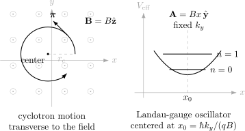
A uniform field separates the physics into cyclotron motion and a guiding-center label. In Landau gauge, fixing $k_y$ turns the transverse Hamiltonian into an oscillator centered at $x_0=\hbar k_y/(qB)$.

Minimal-Coupling Hamiltonian

Minimal coupling replaces canonical momentum by kinetic momentum:

$$\hat{\boldsymbol\pi} = \hat{\mathbf p} - q\mathbf A, \qquad \hat{\mathbf p} = -i\hbar\nabla .$$

With $\Phi=0$, the Hamiltonian is

$$\hat H = \frac{\hat{\boldsymbol\pi}^{\,2}}{2m} = \frac{1}{2m} \left( \hat{\mathbf p}-q\mathbf A \right)^2 .$$

The vector potential is not unique. Two standard choices for $\mathbf B=B\hat{\mathbf z}$ are:

$$\mathbf A_L = Bx\,\hat{\mathbf y} \qquad \text{Landau gauge},$$

and

$$\mathbf A_S = \frac12\mathbf B\times\mathbf r = \frac{B}{2} \left( -y\,\hat{\mathbf x} + x\,\hat{\mathbf y} \right) \qquad \text{symmetric gauge}.$$

Both satisfy

$$\nabla\times\mathbf A = B\hat{\mathbf z}.$$

The two gauges make different symmetries convenient. Landau gauge keeps translation invariance along one transverse direction. Symmetric gauge keeps rotation symmetry around the $z$ axis. Gauge transformations explain why these different-looking descriptions represent the same physical magnetic field.

Kinetic Momentum Algebra

The transverse kinetic momenta are

$$\hat\pi_x = \hat p_x-qA_x, \qquad \hat\pi_y = \hat p_y-qA_y.$$

For a uniform field,

$$[\hat\pi_x,\hat\pi_y] = i\hbar qB .$$

This is the algebraic reason a magnetic field changes the spectrum. Free-particle momenta commute; transverse kinetic momenta in a magnetic field do not. Their noncommutativity is proportional to the magnetic field itself.

The transverse Hamiltonian is

$$\hat H_\perp = \frac{1}{2m} \left( \hat\pi_x^2+\hat\pi_y^2 \right).$$

Introduce the magnetic length

$$\ell_B = \sqrt{ \frac{\hbar}{\lvert q\rvert B} }$$

and the sign

$$s = \operatorname{sgn}(qB).$$

Then the operator

$$\hat a = \frac{\ell_B}{\sqrt2\,\hbar} \left( \hat\pi_x+i s\hat\pi_y \right)$$

satisfies

$$[\hat a,\hat a^\dagger]=1.$$

Moreover,

$$\hat H_\perp = \hbar\omega_c \left( \hat a^\dagger\hat a+\frac12 \right).$$

This is the central setup result: the transverse kinetic motion has the same algebra as a one-dimensional harmonic oscillator. The magnetic field creates the oscillator algebra without introducing an ordinary position-dependent potential.

Landau-Gauge Reduction

In Landau gauge,

$$\mathbf A_L = Bx\,\hat{\mathbf y},$$

the two-dimensional transverse Hamiltonian becomes

$$\hat H_\perp = \frac{1}{2m} \left[ \hat p_x^2 + \left( \hat p_y-qBx \right)^2 \right].$$

This Hamiltonian has no explicit $y$ dependence, so $\hat p_y$ commutes with $\hat H_\perp$. If

$$\psi(x,y) = e^{ik_y y}\varphi(x),$$

then $\hat p_y$ acts as multiplication by $\hbar k_y$, and the $x$ equation contains

$$\left( \hbar k_y-qBx \right)^2 = (qB)^2 \left( x-\frac{\hbar k_y}{qB} \right)^2 .$$

Thus each value of $k_y$ gives a harmonic oscillator in $x$, centered at

$$x_0 = \frac{\hbar k_y}{qB}.$$

The sign of $x_0$ depends on the charge convention, but the oscillator frequency is the positive quantity $\omega_c=\lvert q\rvert B/m$.

This derivation also hints at degeneracy: changing $k_y$ shifts the oscillator center without changing the oscillator frequency. The full counting of allowed centers is part of Landau Levels.

Symmetric-Gauge View

In symmetric gauge,

$$\mathbf A_S = \frac{B}{2} \left( -y\,\hat{\mathbf x} + x\,\hat{\mathbf y} \right),$$

the Hamiltonian does not single out the $x$ or $y$ direction. Instead, rotations about $\hat{\mathbf z}$ are natural. This gauge is useful when angular momentum, circular orbits, or disk geometry matters.

The symmetric-gauge wavefunctions look different from the Landau-gauge wavefunctions. Their labels also look different. This is not a physical disagreement. Gauge-invariant quantities, such as the magnetic field, energy spectrum, local density after a complete degenerate subspace is handled consistently, and physical currents, agree.

Three-Dimensional Motion

For a particle in three dimensions, the uniform magnetic field affects the transverse motion but leaves the longitudinal kinetic energy free:

$$\hat H = \hat H_\perp + \frac{\hat p_z^2}{2m}.$$

This separation is important. Landau quantization is not ordinary confinement in all directions. In the ideal infinite three-dimensional problem, the transverse energy is quantized while the $z$ direction remains continuous. Extra potentials, boundaries, lattice structure, or finite-size conditions can change that statement.

Magnetic Length and Flux Scale

The magnetic length

$$\ell_B = \sqrt{ \frac{\hbar}{\lvert q\rvert B} }$$

is the natural transverse quantum length scale. Stronger magnetic fields make $\ell_B$ smaller and the cyclotron spacing larger:

$$\hbar\omega_c = \frac{\hbar\lvert q\rvert B}{m}.$$

The area scale

$$2\pi\ell_B^2 = \frac{h}{\lvert q\rvert B}$$

is tied to one flux quantum through the plane. This is why the later degeneracy count can be expressed as flux through the sample divided by a flux quantum. This page only identifies the scale; the finite-area state counting is the responsibility of the Landau-level degeneracy discussion.

Physical Interpretation

The useful mental split is:

• kinetic cyclotron motion, which is oscillator-like and carries the energy;
• guiding-center information, which labels where the orbit is centered and accounts for degeneracy in an extended system;
• free longitudinal motion, if the particle is allowed to move along $\mathbf B$.

In Landau gauge, the guiding-center information appears through $k_y$ and $x_0$. In symmetric gauge, it appears through angular structure. Neither label should be mistaken for a universal gauge-invariant observable. The physical statements are the magnetic field, the kinetic energy scale, the magnetic length, and gauge-invariant currents or densities.

Common Mistakes

• Treating $\hat{\mathbf p}$ as the mechanical momentum after a vector potential is introduced.
• Forgetting that $\omega_c$ is positive even when $q$ is negative.
• Thinking the magnetic field creates an ordinary scalar potential well in the transverse plane.
• Comparing Landau-gauge and symmetric-gauge wavefunctions without applying the appropriate gauge transformation.
• Treating $k_y$ in Landau gauge as a universal physical momentum rather than a convenient gauge-dependent label.
• Forgetting that a three-dimensional uniform-field problem remains free along the field direction.
• Including electron spin effects in the spinless Landau setup without saying so.

Exercises

1. Verify that the Landau and symmetric gauges both produce $\mathbf B=B\hat{\mathbf z}$.

Solution

For Landau gauge,

$$A_x=0, \qquad A_y=Bx, \qquad A_z=0.$$

Thus

$$(\nabla\times\mathbf A_L)_z = \frac{\partial A_y}{\partial x} - \frac{\partial A_x}{\partial y} = B,$$

and the other components vanish.

For symmetric gauge,

$$A_x=-\frac{B}{2}y, \qquad A_y=\frac{B}{2}x, \qquad A_z=0.$$

Then

$$(\nabla\times\mathbf A_S)_z = \frac{\partial A_y}{\partial x} - \frac{\partial A_x}{\partial y} = \frac{B}{2} - \left( -\frac{B}{2} \right) = B,$$

with zero $x$ and $y$ components.

2. Derive the commutator $[\hat\pi_x,\hat\pi_y]=i\hbar qB$ in Landau gauge.

Solution

In Landau gauge,

$$\hat\pi_x=\hat p_x, \qquad \hat\pi_y=\hat p_y-qBx.$$

Therefore

$$[\hat\pi_x,\hat\pi_y] = [\hat p_x,\hat p_y] - qB[\hat p_x,x].$$

The first commutator vanishes and

$$[\hat p_x,x] = -i\hbar.$$

Hence

$$[\hat\pi_x,\hat\pi_y] = i\hbar qB.$$

3. Show that the transverse kinetic Hamiltonian has oscillator form.

Solution

Let

$$\hat a = \frac{\ell_B}{\sqrt2\,\hbar} \left( \hat\pi_x+i s\hat\pi_y \right), \qquad s=\operatorname{sgn}(qB).$$

Using

$$[\hat\pi_x,\hat\pi_y] = i s\frac{\hbar^2}{\ell_B^2},$$

one finds

$$[\hat a,\hat a^\dagger]=1.$$

Also,

$$\hat a^\dagger\hat a = \frac{\ell_B^2}{2\hbar^2} \left( \hat\pi_x^2+\hat\pi_y^2 - \frac{\hbar^2}{\ell_B^2} \right).$$

Solving for $\hat\pi_x^2+\hat\pi_y^2$ gives

$$\frac{\hat\pi_x^2+\hat\pi_y^2}{2m} = \frac{\hbar^2}{m\ell_B^2} \left( \hat a^\dagger\hat a+\frac12 \right).$$

Since

$$\frac{\hbar^2}{m\ell_B^2} = \hbar\omega_c,$$

the transverse Hamiltonian is

$$\hat H_\perp = \hbar\omega_c \left( \hat a^\dagger\hat a+\frac12 \right).$$

4. In Landau gauge, explain why changing $k_y$ shifts the oscillator center but not the oscillator frequency.

Solution

With $\psi=e^{ik_y y}\varphi(x)$,

$$\left( \hat p_y-qBx \right)^2 \to \left( \hbar k_y-qBx \right)^2.$$

Completing the square gives

$$\left( \hbar k_y-qBx \right)^2 = (qB)^2 \left( x-\frac{\hbar k_y}{qB} \right)^2 .$$

The center is

$$x_0 = \frac{\hbar k_y}{qB},$$

so changing $k_y$ changes the center. The quadratic coefficient is $(qB)^2/(2m)$, which corresponds to the same positive frequency $\omega_c=\lvert q\rvert B/m$ for every $k_y$.

Where This Is Used

• Landau Levels turn this setup into the full spectrum, wavefunctions, magnetic length interpretation, and degeneracy count.
• Magnetic Translations gives the symmetry algebra behind uniform-field guiding-center degeneracy.
• Landau Gauge and Symmetric Gauge compares the two standard basis choices for the same uniform-field problem.
• Degeneracy of Landau Levels explains why the guiding-center labels produce one state per flux quantum.
• Charged Harmonic Oscillator in a Magnetic Field adds parabolic confinement to the magnetic oscillator setup.
• Minimal Coupling in Wave Mechanics supplies the Hamiltonian and kinetic-momentum conventions.
• Gauge Transformations: First Encounter explains why Landau and symmetric gauges describe the same physical field.
• Quantum Harmonic Oscillator is the canonical home for the oscillator spectrum used after the magnetic reduction.
• Dimensionless Variables and Scaling records $\ell_B$ and $\omega_c$ as natural magnetic scales.
• Probability Current gives the gauge-covariant current needed for physical interpretation.
• Density of States: First Encounter provides the ordinary free-particle state-counting contrast.

References

• D. J. Griffiths and D. F. Schroeter, Introduction to Quantum Mechanics, 3rd ed., Cambridge University Press, 2018.
• R. Shankar, Principles of Quantum Mechanics, 2nd ed., Springer, 1994.
• L. D. Landau and E. M. Lifshitz, Quantum Mechanics: Non-Relativistic Theory, 3rd ed., Pergamon, 1977.
• J. J. Sakurai and J. Napolitano, Modern Quantum Mechanics, 3rd ed., Cambridge University Press, 2020.
• R. E. Prange and S. M. Girvin, eds., The Quantum Hall Effect, 2nd ed., Springer, 1990.