Landau Gauge and Symmetric Gauge

Landau gauge and symmetric gauge are two standard vector-potential choices for the same uniform magnetic field. They lead to different-looking wavefunctions and different convenient quantum numbers, but they do not describe different physics.

For a spinless particle of mass $m$ and charge $q$ in

$$\mathbf B = B\hat{\mathbf z}, \qquad B\gt0,$$

the Hamiltonian is

$$\hat H_\perp = \frac{1}{2m} \left( \hat{\mathbf p}-q\mathbf A \right)^2$$

for the transverse motion. The energy spectrum and degeneracy are derived in Landau Levels. This page explains how the two common gauges organize the same degenerate Hilbert space.

Same Field, Different Potentials

The two most common choices are

$$\mathbf A_L = Bx\,\hat{\mathbf y} \qquad \text{Landau gauge},$$

and

$$\mathbf A_S = \frac12\mathbf B\times\mathbf r = \frac{B}{2} \left( -y\,\hat{\mathbf x} + x\,\hat{\mathbf y} \right) \qquad \text{symmetric gauge}.$$

Both have

$$\nabla\times\mathbf A_L = \nabla\times\mathbf A_S = B\hat{\mathbf z}.$$

Their difference is a gradient:

$$\mathbf A_L-\mathbf A_S = \nabla\left( \frac{Bxy}{2} \right).$$

Thus the gauge function connecting symmetric gauge to Landau gauge is

$$\chi = \frac{Bxy}{2},$$

and wavefunctions transform as

$$\psi_L = \exp\left( \frac{iqBxy}{2\hbar} \right) \psi_S .$$

This phase matters when comparing formulas. It is not correct to place a Landau-gauge wavefunction and a symmetric-gauge wavefunction side by side and demand that they be equal pointwise.

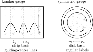
Landau gauge is adapted to strip or rectangular geometry: $k_y$ labels guiding centers $x_0$. Symmetric gauge is adapted to disk geometry: angular labels organize orbitals by radius and rotation.

Landau Gauge

In Landau gauge,

$$\mathbf A_L=Bx\,\hat{\mathbf y},$$

the transverse Hamiltonian is

$$\hat H_\perp = \frac{1}{2m} \left[ \hat p_x^2 + \left( \hat p_y-qBx \right)^2 \right].$$

The Hamiltonian has no explicit $y$ dependence, so

$$[\hat H_\perp,\hat p_y]=0.$$

It is natural to use states of the form

$$\psi_{n,k_y}(x,y) = \frac{e^{ik_y y}}{\sqrt{L_y}} \varphi_n(x-x_0), \qquad x_0 = \frac{\hbar k_y}{qB}.$$

Here $\varphi_n$ is a harmonic-oscillator wavefunction of width $\ell_B$. Explicitly,

$$\varphi_n(x-x_0) = \frac{1}{ \pi^{1/4} \sqrt{2^n n!\,\ell_B} } H_n\left( \frac{x-x_0}{\ell_B} \right) \exp\left[ - \frac{(x-x_0)^2}{2\ell_B^2} \right].$$

The label $k_y$ changes the center $x_0$ but not the energy. This is why Landau gauge makes the guiding-center degeneracy especially transparent in a rectangular sample.

Landau gauge is often the cleanest choice for:

• long strips or rectangles;
• edges parallel to the $y$ direction;
• problems with translation symmetry in one direction;
• calculations where guiding-center position should be visible.

The price is that rotation symmetry is hidden. A circular sample can still be described in Landau gauge, but the basis does not match the geometry.

Symmetric Gauge

In symmetric gauge,

$$\mathbf A_S = \frac{B}{2} \left( -y\,\hat{\mathbf x} + x\,\hat{\mathbf y} \right),$$

the Hamiltonian treats $x$ and $y$ symmetrically. Since $\nabla\cdot\mathbf A_S=0$, expansion gives

$$\hat H_\perp = \frac{\hat p_x^2+\hat p_y^2}{2m} + \frac{q^2B^2}{8m} \left( x^2+y^2 \right) - \frac{qB}{2m}\hat L_z,$$

where

$$\hat L_z = x\hat p_y-y\hat p_x.$$

This form makes rotational symmetry explicit. The transverse Hamiltonian commutes with $\hat L_z$:

$$[\hat H_\perp,\hat L_z]=0.$$

It is natural to write wavefunctions as

$$\psi_{n,m}(r,\phi) = e^{im\phi}R_{n,m}(r), \qquad m\in\mathbb Z,$$

with the allowed and normalizable combinations determined by the Landau-level index and the sign of $qB$.

For one common charge-sign convention, lowest-level states have the schematic form

$$\psi_m(r,\phi) \propto \left( \frac{r}{\ell_B} \right)^m e^{im\phi} \exp\left( - \frac{r^2}{4\ell_B^2} \right), \qquad m=0,1,2,\ldots .$$

For the opposite sign of $qB$, the angular dependence is complex conjugated. The important point is not the convention but the structure: symmetric gauge organizes the degeneracy by angular behavior and radial extent.

Symmetric gauge is often the cleanest choice for:

• disks and circular droplets;
• angular-momentum selection rules;
• quantum Hall orbitals in rotationally symmetric geometry;
• problems where the guiding-center radius is more natural than a Cartesian center coordinate.

The price is that translation symmetry is hidden. A strip problem can still be described in symmetric gauge, but the basis does not match the boundary.

Same Spectrum, Different Basis

The two gauges give the same Landau-level energies:

$$E_n = \hbar\omega_c \left( n+\frac12 \right), \qquad \omega_c = \frac{\lvert q\rvert B}{m}.$$

The wavefunctions are different representatives of the same physical state space. More precisely, each gauge gives a basis for the same Landau-level subspaces, and the bases are related by a gauge phase together with a change of basis inside the degenerate subspace.

This last phrase matters. A single Landau-gauge state localized near one $x_0$ does not usually correspond to a single symmetric-gauge angular-momentum state. Because each Landau level is degenerate, changing from one convenient basis to another can mix labels inside the same energy subspace.

Gauge-invariant quantities include:

• the magnetic field $\mathbf B$;
• the kinetic energy spectrum;
• probabilities and currents when wavefunctions are transformed consistently;
• total state counts in a finite region after boundary conditions are specified;
• expectation values of properly defined physical observables.

Gauge-dependent quantities include:

• the vector potential itself;
• the pointwise phase convention of a wavefunction;
• the convenient canonical momentum label in a chosen gauge;
• the basis used to span a degenerate Landau level.

Degeneracy Labels

In Landau gauge, degeneracy is usually labeled by $k_y$ or by the guiding-center coordinate

$$x_0 = \frac{\hbar k_y}{qB}.$$

For a finite rectangle, allowed $k_y$ values give a sequence of guiding centers. Counting the centers that fit inside the sample leads to the usual flux degeneracy.

In symmetric gauge, degeneracy is usually labeled by angular structure. In a disk, larger angular labels place weight farther from the origin. For the lowest-level schematic state above, the radial probability is concentrated near a radius of order

$$r_m \sim \sqrt{2m}\,\ell_B$$

for large $m$. Requiring such orbitals to fit inside a disk gives the same bulk degeneracy density as the rectangular Landau-gauge count.

The exact finite-size counting depends on boundary conditions and on how sharply the edge is imposed. The physical bulk result is independent of the gauge, but the finite-basis bookkeeping can look quite different.

Choosing a Gauge

A good gauge choice matches the symmetry and boundary conditions of the calculation.

Use Landau gauge when one direction is translation invariant or when a straight edge is central. The label $k_y$ then behaves as a useful bookkeeping variable for guiding centers.

Use symmetric gauge when rotations are central. The angular label then organizes states by their behavior around the origin.

Neither choice is more physical. A gauge that makes one problem transparent can make another problem clumsy. The discipline is to use the convenient description while keeping the final statements gauge invariant.

Common Mistakes

• Thinking that Landau gauge and symmetric gauge describe different magnetic fields.
• Comparing wavefunctions from different gauges without the gauge phase.
• Treating $k_y$ or $m$ as a universal observable rather than a basis label.
• Forgetting that degeneracy allows a change of basis inside a fixed Landau level.
• Assuming a density pattern of one basis state is the density of a filled Landau level.
• Using a gauge adapted to the wrong geometry and then mistaking the algebraic mess for new physics.

Exercises

1. Verify the gauge function connecting symmetric gauge to Landau gauge.

Solution

The difference is

$$\mathbf A_L-\mathbf A_S = Bx\,\hat{\mathbf y} - \frac{B}{2} \left( -y\,\hat{\mathbf x} + x\,\hat{\mathbf y} \right).$$

Therefore

$$\mathbf A_L-\mathbf A_S = \frac{B}{2} \left( y\,\hat{\mathbf x} + x\,\hat{\mathbf y} \right).$$

But

$$\nabla\left( \frac{Bxy}{2} \right) = \frac{B}{2} \left( y\,\hat{\mathbf x} + x\,\hat{\mathbf y} \right).$$

So $\chi=Bxy/2$ connects the two gauges.

2. Expand the symmetric-gauge Hamiltonian and identify the angular-momentum term.

Solution

In symmetric gauge,

$$A_x=-\frac{B}{2}y, \qquad A_y=\frac{B}{2}x.$$

Since $\nabla\cdot\mathbf A_S=0$,

$$\left( \hat{\mathbf p}-q\mathbf A_S \right)^2 = \hat p_x^2+\hat p_y^2 - 2q\mathbf A_S\cdot\hat{\mathbf p} + q^2A_S^2.$$

Now

$$\mathbf A_S\cdot\hat{\mathbf p} = \frac{B}{2} \left( -y\hat p_x+x\hat p_y \right) = \frac{B}{2}\hat L_z,$$

and

$$A_S^2 = \frac{B^2}{4} \left( x^2+y^2 \right).$$

Dividing by $2m$ gives

$$\hat H_\perp = \frac{\hat p_x^2+\hat p_y^2}{2m} + \frac{q^2B^2}{8m} \left( x^2+y^2 \right) - \frac{qB}{2m}\hat L_z.$$

3. Explain why a single Landau-gauge state need not equal a single symmetric-gauge state.

Solution

Each Landau level is degenerate. Landau gauge chooses a basis adapted to translation along $y$, with states labeled by $k_y$ and guiding centers $x_0$. Symmetric gauge chooses a basis adapted to rotations, with states labeled by angular behavior.

Changing gauge multiplies wavefunctions by a position-dependent phase. In addition, changing from one complete basis of a degenerate subspace to another can mix basis labels inside that same subspace. Thus one Landau-gauge basis vector generally expands as a superposition of symmetric-gauge basis vectors within the same Landau level.

4. Which gauge would you choose for a rectangular Hall bar with straight edges parallel to $y$? Which would you choose for a circular droplet?

Solution

For the rectangular Hall bar, Landau gauge is usually convenient because translation along $y$ is built into the basis and $k_y$ labels guiding centers across the width.

For a circular droplet, symmetric gauge is usually convenient because rotations around the center are built into the basis and angular labels organize the orbitals naturally.

Where This Is Used

• Landau Levels provides the spectrum and degeneracy result whose gauge representations are compared here.
• Degeneracy of Landau Levels gives the canonical finite-area count behind the guiding-center and angular labels.
• Charged Harmonic Oscillator in a Magnetic Field uses symmetric gauge to combine circular oscillator modes with magnetic splitting.
• Particle in a Uniform Magnetic Field sets up the kinetic-momentum algebra and oscillator reduction behind both gauges.
• Gauge Transformations: First Encounter gives the general transformation law for $\mathbf A$ and $\psi$.
• Degeneracy in Separable Systems gives the earlier language for distinguishing accidental, symmetry, and label-based degeneracies.
• Orbital Angular Momentum supplies the $\hat L_z$ operator that symmetric gauge makes useful.
• Momentum Operator records the canonical-versus-kinetic momentum distinction.

References

• D. J. Griffiths and D. F. Schroeter, Introduction to Quantum Mechanics, 3rd ed., Cambridge University Press, 2018.
• R. Shankar, Principles of Quantum Mechanics, 2nd ed., Springer, 1994.
• L. D. Landau and E. M. Lifshitz, Quantum Mechanics: Non-Relativistic Theory, 3rd ed., Pergamon, 1977.
• J. J. Sakurai and J. Napolitano, Modern Quantum Mechanics, 3rd ed., Cambridge University Press, 2020.
• R. E. Prange and S. M. Girvin, eds., The Quantum Hall Effect, 2nd ed., Springer, 1990.