Degeneracy of Landau Levels

An ideal Landau level is highly degenerate. In a finite two-dimensional region of area $A$, each spinless Landau level contains approximately

$$N_\Phi = \frac{A}{2\pi\ell_B^2} = \frac{\lvert q\rvert BA}{h}$$

single-particle states in the bulk. Equivalently, the number of states per unit area is

$$\frac{N_\Phi}{A} = \frac{1}{2\pi\ell_B^2} = \frac{\lvert q\rvert B}{h} = \frac{\lvert q\rvert B}{2\pi\hbar}.$$

This page is the canonical home for the state-counting argument. Landau Levels derives the energy ladder; this page explains how many states live in each rung and why the answer is a flux count.

What Is Being Counted

The ideal model is a spinless nonrelativistic particle of charge $q$ in a uniform magnetic field

$$\mathbf B = B\hat{\mathbf z}, \qquad B\gt0.$$

The transverse kinetic energy has Landau levels

$$E_n = \hbar\omega_c \left( n+\frac12 \right), \qquad n=0,1,2,\ldots .$$

The degeneracy discussed here is the number of independent orbital states with the same $n$ in a finite region. Spin, valley, layer, band, and other internal degeneracies are additional factors only when those degrees of freedom are present and unsplit.

On the infinite plane, the degeneracy is infinite. The meaningful bulk statement is a density of states per area. To derive it, temporarily place the particle in a finite region, count the allowed guiding-center labels, and then take a large-area limit.

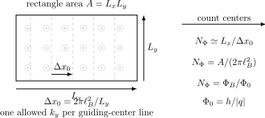
In Landau gauge, adjacent allowed $k_y$ values correspond to guiding centers separated by $\Delta x_0=2\pi\ell_B^2/L_y$. Counting centers in width $L_x$ gives one state per area $2\pi\ell_B^2$, equivalently one state per flux quantum.

Landau-Gauge Count

Take a rectangle of area

$$A=L_xL_y$$

and use Landau gauge

$$\mathbf A = Bx\,\hat{\mathbf y}.$$

The Landau-gauge states have the form

$$\psi_{n,k_y}(x,y) = \frac{e^{ik_y y}}{\sqrt{L_y}} \varphi_n(x-x_0), \qquad x_0 = \frac{\hbar k_y}{qB}.$$

The sign of $qB$ controls whether increasing $k_y$ moves the center to larger or smaller $x$. The spacing of centers depends only on the magnitude.

Impose periodic boundary conditions along $y$:

$$k_y = \frac{2\pi r}{L_y}, \qquad r\in\mathbb Z.$$

Adjacent $k_y$ values differ by

$$\Delta k_y = \frac{2\pi}{L_y}.$$

Therefore adjacent guiding centers are separated by

$$\Delta x_0 = \frac{\hbar\,\Delta k_y}{\lvert q\rvert B} = \frac{2\pi\hbar}{\lvert q\rvert BL_y} = \frac{2\pi\ell_B^2}{L_y}.$$

The number of centers that fit inside a width $L_x$ is approximately

$$N_\Phi = \frac{L_x}{\Delta x_0} = \frac{L_xL_y}{2\pi\ell_B^2} = \frac{A}{2\pi\ell_B^2}.$$

This is the bulk degeneracy of one spinless Landau level in area $A$. The approximation becomes sharp away from boundaries when the region is large compared with $\ell_B$.

Flux Form

Using

$$\ell_B^2 = \frac{\hbar}{\lvert q\rvert B},$$

the count becomes

$$N_\Phi = \frac{\lvert q\rvert BA}{2\pi\hbar} = \frac{\lvert q\rvert BA}{h}.$$

The magnetic flux through the rectangle is

$$\Phi_B = BA.$$

For a particle of charge magnitude $\lvert q\rvert$, define the flux quantum

$$\Phi_0 = \frac{h}{\lvert q\rvert}.$$

Then

$$N_\Phi = \frac{\Phi_B}{\Phi_0}$$

for the orientation convention $B\gt0$. More invariantly, the bulk count is controlled by $\lvert q\Phi_B\rvert/h$.

This formula should be read as a single-particle orbital count for the charge used in the Hamiltonian. For superconducting flux quantization, the relevant charge is that of a Cooper pair, so the conventional flux quantum differs by a factor of two from the electron single-particle value.

Guiding-Center Algebra

The degeneracy is not a mysterious extra copy of the oscillator. It comes from a second pair of operators: the guiding-center coordinates. In two dimensions define

$$\hat X = \hat x+\frac{\hat\pi_y}{qB}, \qquad \hat Y = \hat y-\frac{\hat\pi_x}{qB}.$$

In Landau gauge, $\hat X$ becomes the oscillator-center coordinate $x_0$ on a state with definite $k_y$:

$$\hat X \to \frac{\hbar k_y}{qB}.$$

The guiding-center coordinates commute with the transverse Hamiltonian but not with each other:

$$[\hat X,\hat Y] = -\frac{i\hbar}{qB} = -i\,\operatorname{sgn}(qB)\,\ell_B^2.$$

Thus the guiding center behaves like its own noncommuting phase plane. A region of ordinary area $A$ supports roughly one independent guiding-center state per area $2\pi\ell_B^2$, just as a canonical phase space supports one quantum state per area $2\pi\hbar$.

This algebraic explanation is gauge independent. Landau gauge makes $\hat X$ visible as $x_0$; symmetric gauge organizes the same guiding-center space with angular labels.

Symmetric-Gauge Count

In symmetric gauge, lowest-level orbitals are commonly organized by an angular label. Up to charge-sign conventions, their radial weight is concentrated at radii of order

$$r_m \sim \sqrt{2m}\,\ell_B$$

for large $m$. A disk of radius $R$ and area $A=\pi R^2$ can hold angular labels up to roughly

$$m_{\max} \sim \frac{R^2}{2\ell_B^2}.$$

Therefore the number of orbitals is

$$N_\Phi \sim \frac{R^2}{2\ell_B^2} = \frac{\pi R^2}{2\pi\ell_B^2} = \frac{A}{2\pi\ell_B^2}.$$

The disk argument is less convenient for exact finite counting but useful for intuition. Large angular labels live near the edge, while small angular labels live near the center. The same bulk density appears because the two gauges describe the same guiding-center Hilbert space.

Boundary and Topology Caveats

The formula

$$\frac{N_\Phi}{A} = \frac{1}{2\pi\ell_B^2}$$

is a bulk result. Finite systems require boundary conditions.

For a rectangle with periodic boundary conditions in one direction, the Landau-gauge count is approximate unless one specifies exactly how to treat centers near the edges. For a torus with periodic boundary conditions in both directions, consistency of magnetic translations requires the total flux in units of $\Phi_0$ to be an integer. In that setting, the degeneracy of each ideal Landau level is exactly that integer.

Physical samples have edges. Near an edge, the confining potential can bend the energies and produce edge modes. Disorder broadens Landau levels, while interactions change the many-particle problem. None of these effects invalidate the bulk orbital density, but they matter for spectra, transport, and finite-size numerics.

Spin and Internal Degeneracy

The count above is orbital and spinless. If an electron spin degree of freedom is included and Zeeman splitting is neglected, each orbital Landau level can carry an additional factor of two:

$$N_{\mathrm{states}} = 2N_\Phi.$$

If Zeeman splitting is included, the spin-up and spin-down energies separate, and the simple factor of two is no longer a degeneracy at fixed energy. The same logic applies to valley, layer, subband, or other internal labels: multiply only when the Hamiltonian actually leaves them degenerate.

Scale Check

For an electron at $B=1\,\mathrm T$,

$$\ell_B \approx 25.7\,\mathrm{nm},$$

and the spinless degeneracy density is

$$\frac{1}{2\pi\ell_B^2} \approx 2.42\times10^{14}\,\mathrm{m}^{-2} = 2.42\times10^{10}\,\mathrm{cm}^{-2}.$$

These are large but experimentally natural densities. This is why Landau-level filling can be tuned in two-dimensional electron systems by changing magnetic field or carrier density.

Common Mistakes

• Counting $k_y$ values without restricting the guiding centers to the sample.
• Forgetting that the sign of $qB$ reverses the ordering of centers but not the degeneracy density.
• Treating the infinite-plane degeneracy as a finite number without introducing area or boundary conditions.
• Multiplying by spin degeneracy after including Zeeman splitting.
• Confusing the single-particle flux quantum $h/\lvert q\rvert$ with the superconducting flux quantum for charge $2e$.
• Assuming edge states or disorder change the bulk degeneracy density rather than the finite-size spectrum and level broadening.

Exercises

1. Derive the Landau-gauge degeneracy for a rectangle of area $A=L_xL_y$.

Solution

Periodic boundary conditions along $y$ give

$$k_y = \frac{2\pi r}{L_y}.$$

The guiding center is

$$x_0 = \frac{\hbar k_y}{qB}.$$

Neighboring allowed values are separated by

$$\Delta x_0 = \frac{2\pi\ell_B^2}{L_y}$$

in magnitude. The number of centers fitting inside width $L_x$ is therefore

$$N_\Phi = \frac{L_x}{\Delta x_0} = \frac{L_xL_y}{2\pi\ell_B^2} = \frac{A}{2\pi\ell_B^2}.$$

2. Convert the area formula into a flux formula.

Solution

Using

$$\ell_B^2 = \frac{\hbar}{\lvert q\rvert B},$$

we get

$$N_\Phi = \frac{A}{2\pi\ell_B^2} = \frac{\lvert q\rvert BA}{2\pi\hbar} = \frac{\lvert q\rvert BA}{h}.$$

Since $\Phi_B=BA$ and $\Phi_0=h/\lvert q\rvert$,

$$N_\Phi = \frac{\Phi_B}{\Phi_0}$$

for the orientation convention $B\gt0$.

3. Estimate the number of spinless states in one Landau level for a disk of radius $R$.

Solution

The area is

$$A=\pi R^2.$$

The bulk degeneracy is one state per area $2\pi\ell_B^2$, so

$$N_\Phi \approx \frac{\pi R^2}{2\pi\ell_B^2} = \frac{R^2}{2\ell_B^2}.$$

This matches the symmetric-gauge estimate that angular labels fit until $r_m\sim R$.

4. Suppose electron spin is included but Zeeman splitting is negligible. What changes?

Solution

Each orbital state can be occupied with two spin labels. If the Hamiltonian does not split those spin states, the degeneracy at fixed orbital Landau level doubles:

$$N_{\mathrm{states}} = 2N_\Phi.$$

If Zeeman splitting is included, those two spin labels generally have different energies, so they should be counted as separate levels rather than as one degenerate level.

5. Why does a torus require an integer number of flux quanta?

Solution

On a torus, the wavefunction must be consistently defined after translations around both cycles. Magnetic translations around the two cycles fail to commute by a phase proportional to the total magnetic flux. For the boundary conditions to be globally consistent, this phase must be unity. That condition requires

$$\frac{\Phi_B}{\Phi_0} \in \mathbb Z.$$

When this holds, each ideal Landau level has exactly that many orbital states on the torus.

Where This Is Used

• Landau Levels uses this degeneracy to interpret the size of each magnetic energy level.
• Magnetic Translations derives the same flux-counting scale from the noncommuting translation algebra.
• Landau Gauge and Symmetric Gauge compares the two standard ways of labeling the same degenerate subspace.
• Density of States: First Encounter gives the ordinary free-particle counting that magnetic flux counting replaces in two dimensions.
• Dimensionless Variables and Scaling defines the magnetic length used in the area formula.
• Degeneracy in Separable Systems gives the general language for degeneracy before this magnetic example.
• Chern Numbers supplies later topological language used in quantum Hall settings.
• Integer Quantum Hall Effect turns the flux degeneracy into a filling-factor ledger and then adds plateau, edge, and localization physics.

References

• D. J. Griffiths and D. F. Schroeter, Introduction to Quantum Mechanics, 3rd ed., Cambridge University Press, 2018.
• R. Shankar, Principles of Quantum Mechanics, 2nd ed., Springer, 1994.
• L. D. Landau and E. M. Lifshitz, Quantum Mechanics: Non-Relativistic Theory, 3rd ed., Pergamon, 1977.
• J. J. Sakurai and J. Napolitano, Modern Quantum Mechanics, 3rd ed., Cambridge University Press, 2020.
• R. E. Prange and S. M. Girvin, eds., The Quantum Hall Effect, 2nd ed., Springer, 1990.