Integer Quantum Hall Effect

The integer quantum Hall effect is the quantization of transverse electrical response in an effectively two-dimensional electronic system whose bulk is insulating at the Fermi level while chiral boundary channels remain conducting. In a Hall bar at low temperature and strong perpendicular magnetic field, the Hall resistance develops broad plateaus while the longitudinal resistance becomes very small:

$$\left|R_{yx}\right| = \frac{h}{\nu e^2}, \qquad R_{xx}\simeq0, \qquad \nu\in\mathbb N.$$

The striking feature is not merely that an ideal Landau-level model produces an integer. It is that a disordered, finite device with contacts can reproduce the same resistance over a finite interval of magnetic field or carrier density. Landau quantization supplies the levels, topology fixes the transverse response, localized bulk states widen the plateaus, and chiral edge channels connect that bulk response to a multiprobe measurement.

This page owns the integer material phenomenon: its experimental signature, filling factor, plateau mechanism, edge transport, precision, and interpretation. Fractional Quantum Hall Effect owns the interaction-driven Hall fluid, Laughlin state, fractional charge, anyonic statistics, composite fermions, and fractional edges. Topology in Quantum Matter owns the general gapped-phase, protection, boundary, and response ledger. Landau Levels owns the single-particle spectrum, Degeneracy of Landau Levels owns flux counting, Hall Effect owns classical and anomalous Hall transport, Chern Numbers owns the geometric invariant, and Chern Numbers in Band Theory owns its occupied-projector, Kubo, and numerical band realization.

Required background. Landau Levels supplies the spectrum, Degeneracy of Landau Levels supplies flux counting, and Hall Effect supplies the Hall-tensor and transport definitions.

Helpful background. Topology in Quantum Matter supplies the phase and evidence ledger, Chern Numbers and Chern Numbers in Band Theory supply the geometric and band-projector formulations, and Kubo Formula supplies the general response derivation.

Convention Ledger

Take a right-handed $(x,y,z)$ frame, a two-dimensional sample in the $xy$ plane, and

$$\mathbf B=B\hat{\mathbf z}, \qquad B>0.$$

The mobile particles are electrons of charge $q=-e$, where $e>0$. As on the Hall Effect page, write

$$\begin{pmatrix} j_x\\ j_y \end{pmatrix} = \begin{pmatrix} \sigma_{xx} & \sigma_{xy}\\ -\sigma_{xy} & \sigma_{xx} \end{pmatrix} \begin{pmatrix} E_x\\ E_y \end{pmatrix}.$$

The inverse tensor gives

$$\rho_{xx} = \frac{\sigma_{xx}} {\sigma_{xx}^2+\sigma_{xy}^2}, \qquad \rho_{yx} = \frac{\sigma_{xy}} {\sigma_{xx}^2+\sigma_{xy}^2}.$$

For an ideal two-dimensional Hall bar, $\rho_{yx}$ is a sheet resistance and may be identified with the four-terminal Hall resistance after the lead polarity has been declared. On a plateau,

$$\sigma_{xx}\to0 \quad\Longrightarrow\quad \rho_{yx}=\frac{1}{\sigma_{xy}}, \qquad \rho_{xx}\to0.$$

For electrons with $B>0$, the convention above normally gives $\sigma_{xy}<0$. To keep the universal magnitudes visible while avoiding silent sign changes between common tensor conventions, this page writes

$$\left|\sigma_{xy}\right| = \nu\frac{e^2}{h}, \qquad \left|\rho_{yx}\right| = \frac{h}{\nu e^2}.$$

Signed formulas are stated explicitly when needed. Reversing $B$, reversing the carrier charge, reversing the orientation of the sample, or exchanging the tensor-index convention reverses the Hall sign but not the quantized magnitude.

Experimental Signature

The original observation used a silicon metal–oxide–semiconductor field-effect transistor, where a gate confines electrons to an inversion layer. Modern platforms include GaAs/AlGaAs heterostructures, graphene, oxide interfaces, and other effectively two-dimensional conductors. Material details change the accessible temperatures, fields, degeneracies, and plateau sequence, but the diagnostic logic is the same.

A four-terminal measurement separates the imposed current path from the voltage probes. As magnetic field or carrier density is swept:

1. $R_{yx}$ becomes nearly constant on a plateau;
2. $R_{xx}$ develops a deep minimum in the same interval;
3. transitions between adjacent plateaus coincide with peaks in $R_{xx}$;
4. the plateau value approaches $R_K/\nu$, where $R_K=h/e^2$;
5. the result is independent of the macroscopic aspect ratio after the Hall-bar geometry and lead configuration are treated correctly.

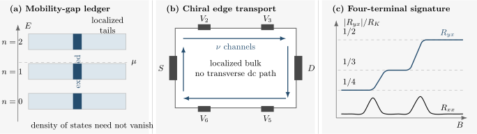
Three complementary ledgers for the integer quantum Hall effect. Disorder broadens each Landau level into localized tails around a narrow band of current-carrying extended states. In a Hall bar, $\nu$ chiral channels connect contacts around the boundary. When the chemical potential lies in a mobility gap, $R_{yx}/R_K$ is pinned to $1/\nu$ while $R_{xx}$ is small; crossing extended states produces a plateau transition and a longitudinal peak.

A low value of $R_{xx}$ alone is not enough. A short circuit, a superconducting path, contact failure, or an incorrectly symmetrized trace can also produce a small longitudinal voltage. Reliable identification requires the correlated Hall plateau, field-reversal checks, current-reversal checks, stable contacts, and a regime below quantum Hall breakdown.

Landau Levels and Filling Factor

For one resolved internal component, each Landau level contains

$$N_\Phi = \frac{BA}{\Phi_e}, \qquad \Phi_e = \frac{h}{e}$$

orbital states in area $A$, up to finite-boundary corrections. Equivalently, the degeneracy per unit area is

$$n_\Phi = \frac{N_\Phi}{A} = \frac{eB}{h} = \frac{1}{2\pi\ell_B^2}, \qquad \ell_B = \sqrt{\frac{\hbar}{eB}}.$$

For electron sheet density $n_{2\mathrm D}$, the filling factor is

$$\nu \equiv \frac{N_{\mathrm e}}{N_\Phi} = \frac{n_{2\mathrm D}h}{eB} = 2\pi\ell_B^2n_{2\mathrm D}.$$

In the simplest spin-resolved continuum model, integer $\nu$ counts completely occupied Landau levels. The orbital energies are

$$E_n = \hbar\omega_c \left( n+\frac12 \right), \qquad \omega_c = \frac{eB}{m}.$$

Real systems also have Zeeman, valley, layer, subband, and interaction-induced splittings. A convenient one-electron bookkeeping model is

$$E_{n,s} = \hbar\omega_c \left( n+\frac12 \right) + s\,g^\ast\mu_BB, \qquad s=\pm\frac12.$$

Whether neighboring spin branches are resolved depends on the effective $g$ factor, interaction enhancement, disorder broadening, and temperature. Consequently, not every material shows every positive integer in the same field range. In graphene, the Dirac spectrum and spin–valley structure produce a different sequence from a parabolic single-valley two-dimensional electron gas. The integer $\nu$ must therefore be inferred from the full degeneracy ledger, not guessed from an orbital index alone.

A useful counting check

If exactly $\nu$ resolved levels are filled, then

$$n_{2\mathrm D} = \nu\frac{eB}{h}.$$

Inserting this into the magnitude of the classical one-carrier Hall result gives

$$\left|\rho_{yx}\right| = \frac{B}{en_{2\mathrm D}} = \frac{h}{\nu e^2}.$$

This agreement is an important consistency check, but it is not an explanation of precision or plateau width. In a perfectly clean system at fixed density, exact integer filling occurs only at isolated magnetic fields. Flux counting predicts the value at those fields; localization and topology explain why the measured value remains pinned while $B$ or $n_{2\mathrm D}$ changes.

Chiral Edge States

A confining potential turns the macroscopically degenerate bulk levels into dispersing states near a boundary. In Landau gauge, a momentum label fixes a guiding-center coordinate $Y$. If the confining potential $U(Y)$ varies slowly on the magnetic-length scale, the edge dispersion is approximately

$$E_n(k) \simeq \hbar\omega_c \left( n+\frac12 \right) + U(Y_k).$$

The group velocity is

$$v_n(k) = \frac{1}{\hbar} \frac{dE_n}{dk} \simeq \frac{1}{\hbar} \frac{dU}{dY} \frac{dY_k}{dk}.$$

The confining potential has opposite slope on opposite sides of a Hall bar. Thus the modes propagate in opposite coordinate directions on opposite edges, yet together circulate with one chirality around the sample boundary. At a given edge there is no nearby mode moving backward at the same energy in the ideal integer regime.

For one perfectly transmitted one-dimensional channel connecting reservoirs at electrochemical potentials $\mu_S$ and $\mu_D$, the Landauer current is

$$I_1 = \frac{e}{h} \int_{\mu_D}^{\mu_S}dE = \frac{e}{h} \left( \mu_S-\mu_D \right).$$

With $\mu_S-\mu_D=eV$ and $\nu$ equilibrated channels,

$$I = \nu\frac{e^2}{h}V.$$

The corresponding conductance magnitude is

$$G = \nu\frac{e^2}{h}.$$

Chirality suppresses elastic backscattering because a carrier cannot reverse direction without reaching a counterpropagating channel, usually on the opposite edge or in another unequilibrated branch. This statement has conditions. Poor contacts, edge reconstruction, interchannel scattering, a narrow sample, strong disorder connecting opposite sides, excessive source–drain current, or nonideal voltage probes can spoil exact multiprobe quantization.

Bulk and edge are complementary

The bulk and edge descriptions answer different parts of the same experiment:

• the bulk Chern number fixes the net number and chirality of boundary modes relative to the exterior;
• localized bulk states allow the chemical potential to move without changing the Hall integer;
• edge channels carry nonequilibrium current between reservoirs;
• contacts populate and equilibrate the incoming channels.

It is therefore misleading to ask whether the Hall current is “really” a bulk current or “really” an edge current without specifying geometry, equilibrium subtraction, and the measured observable. The topological response can be computed with periodic boundaries and no physical edge, while a Hall-bar voltage measurement necessarily involves boundaries and reservoirs.

Laughlin Flux-Insertion Argument

Place the two-dimensional system on a cylinder and thread magnetic flux $\Phi$ through its axis. Increasing the flux by one electronic flux quantum,

$$\Delta\Phi = \Phi_e = \frac{h}{e},$$

returns the Hamiltonian to a gauge-equivalent form. During the insertion, Faraday induction creates an electric field around the cylinder and transports charge from one boundary to the other.

If the process is adiabatic and the mobility gap remains effective, the final state differs by an integer spectral flow. Suppose the net transported charge magnitude is

$$\left|\Delta Q\right| = \nu e.$$

The integrated Hall response also gives

$$\left|\Delta Q\right| = \left|\sigma_{xy}\right| \Delta\Phi.$$

Therefore

$$\left|\sigma_{xy}\right| \frac{h}{e} = \nu e,$$

and hence

$$\left|\sigma_{xy}\right| = \nu\frac{e^2}{h}.$$

The argument isolates the two ingredients behind exact quantization: gauge equivalence after one flux quantum and integer charge spectral flow in a phase that does not become dissipative during the cycle. It does not by itself calculate every plateau sequence or describe localization quantitatively. Those require the microscopic spectrum, internal degeneracies, disorder, and contacts.

Chern Number Interpretation

For clean noninteracting electrons in a periodic two-dimensional system, use the oriented measure $dk_x\wedge dk_y$, the Berry connection $\mathcal A_n=i\langle u_n|\boldsymbol\nabla_{\mathbf k}u_n\rangle$, and $\Omega_n=\partial_{k_x}\mathcal A_{n,y}-\partial_{k_y}\mathcal A_{n,x}$. With the electron and conductivity-tensor conventions above, the Kubo formula can then be reorganized into the Thouless–Kohmoto–Nightingale–den Nijs expression

$$\sigma_{xy} = -\frac{e^2}{h}C_{\mathrm{occ}},$$

where

$$C_{\mathrm{occ}} = \frac{1}{2\pi} \sum_{n\in\mathrm{occ}} \int_{\mathrm{BZ}} \Omega_n(\mathbf k)\,d^2k.$$

The sign of $C_{\mathrm{occ}}$ follows the chosen Brillouin-zone orientation and Berry-curvature convention. With the complete convention block used here, the Chern and Hall signs are opposite: filled continuum electron Landau levels at $B>0$ have $C_{\mathrm{occ}}>0$ and $\sigma_{xy}<0$. Each resolved filled Landau level changes the magnitude of the Hall integer by one. A source using $\mathcal A=-i\langle u|\boldsymbol\nabla_{\mathbf k}u\rangle$ reverses the reported Chern sign and the written bridge together.

The Chern number explains why weak perturbations cannot continuously shift the plateau value. As long as the relevant occupied subspace remains isolated in the appropriate spectral or mobility sense, an integer-valued invariant cannot drift. A plateau transition requires the assumptions defining that invariant to fail, which in a disordered Landau level occurs through delocalized critical states.

Boundary twists when translation symmetry is absent

Ordinary crystal momentum is not available in a disordered sample. Put the many-electron system on a torus and impose twisted boundary conditions

$$\Psi(\ldots,\mathbf r_i+L_\alpha\hat{\boldsymbol\alpha},\ldots) = e^{i\theta_\alpha} \Psi(\ldots,\mathbf r_i,\ldots), \qquad \alpha=x,y.$$

The twist angles form a parameter-space torus,

$$(\theta_x,\theta_y) \in [0,2\pi)\times[0,2\pi).$$

For a nondegenerate gapped many-body ground state, define

$$\mathcal A_\alpha = i \left\langle \Psi_0 \middle| \partial_{\theta_\alpha}\Psi_0 \right\rangle$$

and

$$\mathcal F_{\theta_x\theta_y} = \partial_{\theta_x}\mathcal A_y - \partial_{\theta_y}\mathcal A_x.$$

The many-body Chern number is

$$C_{\mathrm{MB}} = \frac{1}{2\pi} \int_0^{2\pi}d\theta_x \int_0^{2\pi}d\theta_y\, \mathcal F_{\theta_x\theta_y}.$$

This construction generalizes the band invariant to disorder and interactions under suitable gap, locality, and thermodynamic-limit assumptions. In a mobility-gapped integer Hall regime, more refined formulations express the invariant directly in terms of localized projectors. The important conceptual point is that disorder removes crystal momentum, not topological quantization.

Quantum Hall Geometry Preview develops this parameter-space viewpoint. Kubo Formula owns the general linear-response machinery.

Disorder, Localization, and Plateaus

A smooth or weak random potential broadens each ideal Landau level. In the standard noninteracting localization picture:

• states in the disorder-broadened tails are localized in the bulk;
• a narrow region near the center contains extended or critical states;
• the localization length grows toward a critical energy $E_c$;
• crossing $E_c$ changes the Hall integer and produces dissipative longitudinal transport.

Near a plateau transition, the localization length scales as

$$\xi(E) \sim \left| E-E_c \right|^{-\nu_{\mathrm{loc}}},$$

where $\nu_{\mathrm{loc}}$ is a critical exponent, not the filling factor. Finite sample size, finite temperature, and the phase-coherence length cut off the divergence observed experimentally.

Spectral gap versus mobility gap

A spectral gap is an interval with no bulk eigenstates. A mobility gap may contain bulk eigenstates, but those states are localized and cannot support dc transport across a macroscopic sample. Integer Hall plateaus in disordered devices are commonly mobility-gap phenomena.

As $B$ changes at fixed density, localized orbitals can gain or lose occupation without carrying current between contacts. The Hall integer therefore remains fixed while the chemical potential traverses localized states. Only when the chemical potential encounters extended states can charge percolate across the sample, $\sigma_{xx}$ become appreciable, and $\sigma_{xy}$ move to the next plateau.

The useful statement is not “disorder creates quantization.” In a clean gapped system, topology already quantizes the ideal Hall response. Moderate disorder localizes bulk states and converts isolated integer fillings into finite-width plateaus. Strong enough disorder, heating, or electric-field breakdown eventually destroys the mobility gap and the quantized regime.

Finite temperature and breakdown

If the nearest mobility edge is an energy $\delta_{\mathrm{mob}}$ from the chemical potential, thermally activated longitudinal transport can scale approximately as

$$\sigma_{xx}(T) \propto \exp \left( -\frac{\delta_{\mathrm{mob}}}{k_BT} \right)$$

over an activated regime. At lower temperature, hopping among localized states can replace simple activation. At high measurement current, the Hall electric field heats carriers and promotes inter-level or inter-edge processes; $R_{xx}$ rises and the Hall plateau departs from its quantized value. “Low temperature” and “strong field” are therefore operational conditions set by the relevant gaps, disorder, geometry, and allowed current density.

Středa Formula

There is also a thermodynamic route to the Hall response. In a gapped two-dimensional regime where the Fermi-surface contribution vanishes, the Středa relation in this page’s signed convention is

$$\sigma_{xy} = q \left( \frac{\partial n}{\partial B} \right)_\mu,$$

where $q=-e$ for electrons. If the grand-potential density is $\omega(\mu,B)$, then

$$n = -\frac{\partial\omega}{\partial\mu}, \qquad M = -\frac{\partial\omega}{\partial B}.$$

Equality of mixed derivatives gives

$$\left( \frac{\partial n}{\partial B} \right)_\mu = \left( \frac{\partial M}{\partial\mu} \right)_B,$$

so that

$$\sigma_{xy} = q \left( \frac{\partial M}{\partial\mu} \right)_B.$$

For $\nu$ filled electron Landau levels at $B>0$,

$$n = \nu\frac{eB}{h},$$

and hence

$$\sigma_{xy} = (-e) \left( \nu\frac{e}{h} \right) = -\nu\frac{e^2}{h}.$$

The formula makes density response, orbital magnetization, and Hall conductance parts of one thermodynamic ledger. Away from a gap or mobility gap, additional Fermi-surface terms matter; the simple derivative must not be used as a universal metallic Hall formula.

Resistivity Is Not Always a Reciprocal

On a well-developed plateau, $\sigma_{xx}\simeq0$, so $\rho_{yx}\simeq1/\sigma_{xy}$. During a plateau transition,

$$\rho_{yx} = \frac{\sigma_{xy}} {\sigma_{xx}^2+\sigma_{xy}^2}, \qquad \rho_{xx} = \frac{\sigma_{xx}} {\sigma_{xx}^2+\sigma_{xy}^2}.$$

Thus neither $\rho_{yx}=1/\sigma_{xy}$ nor $\rho_{xx}=1/\sigma_{xx}$ is valid when both tensor components are appreciable. This is experimentally important: a peak in $R_{xx}$ and a changing Hall trace must be converted with the full tensor before being compared with conductivity scaling.

Precision and Resistance Metrology

The natural resistance scale is the von Klitzing constant

$$R_K \equiv \frac{h}{e^2}.$$

Using the exact defining values of $h$ and $e$ in the revised SI,

$$R_K = 25\,812.807\,459\,3045\ \Omega$$

is the BIPM-recommended 15-significant-digit value for practical realization. An integer plateau has magnitude

$$\left|R_{yx}\right| = \frac{R_K}{\nu}.$$

Since 20 May 2019, $h$ and $e$ have exact numerical values in SI units, so $h/e^2$ is exact as a derived constant. That does not make every voltage reading on a quantum Hall device exact. A practical realization has uncertainty from contact quality, leakage, thermoelectric offsets, finite $R_{xx}$, device inhomogeneity, current-source error, voltmeter loading, and departure from the plateau.

A metrological measurement therefore verifies a device regime rather than merely substituting constants into a formula. Typical checks include:

Check	What failure would reveal
negligible longitudinal voltage	dissipation or breakdown
plateau flatness versus field or density	proximity to a transition
current reversal	thermoelectric and dc offsets
magnetic-field reversal	lead mixing and odd/even contamination
several contact pairs	inhomogeneity or bad contacts
current below breakdown	carrier heating and interchannel transfer
comparison across devices or materials	failure of universality

The quantum Hall effect realizes resistance because the response is both universal and experimentally reproducible. Traceability still requires a complete uncertainty budget and measurement protocol.

Bridge to Chern–Simons Response

At wavelengths and frequencies too low to resolve Landau levels, localized orbitals, or edge structure, a gapped integer Hall phase can be summarized by an electromagnetic Chern–Simons term. In differential-form notation,

$$S_{\mathrm{eff}}[A] = \frac{C_H e^2}{4\pi\hbar} \int A\wedge dA + \cdots,$$

where $C_H$ is the signed Hall-response level and the omitted terms contain higher derivatives or nonuniversal response. Here $x^0=t$, $\epsilon^{0xy}=+1$, $A_0=-\phi$, and

$$E_i = -\partial_t A_i-\partial_i\phi = -\partial_t A_i+\partial_i A_0.$$

With $j^\mu=\delta S_{\mathrm{eff}}/\delta A_\mu$ in this convention, variation gives

$$j^\mu = \frac{C_H e^2}{2\pi\hbar} \epsilon^{\mu\nu\rho} \partial_\nu A_\rho,$$

whose spatial part contains

$$\sigma_{xy} = C_H\frac{e^2}{h}.$$

This response coefficient is not a second definition of the occupied-band Chern number. With the page-wide electron-charge, Berry-connection, Brillouin-zone-orientation, and Hall-tensor conventions,

$$C_H = -C_{\mathrm{occ}}, \qquad \sigma_{xy} = -C_{\mathrm{occ}}\frac{e^2}{h}.$$

Keeping the distinct symbols prevents the sign carried by the response action from being silently identified with the sign of the occupied-band bundle.

On a space with boundary, the Chern–Simons action is not independently gauge invariant. The boundary variation is canceled by the chiral edge theory: this is the response-theory form of bulk–boundary correspondence.

The effective action records the quantized long-distance response; it does not replace the microscopic explanation of Landau levels, the localization mechanism that makes plateaus broad, or the reservoir physics of a Hall bar. Berry Phase to Topological Terms develops the bridge toward field-theoretic language.

Interpretation Workflow

Use the following sequence when reading an integer quantum Hall data set:

1. Establish effective two-dimensionality. Compare confinement, subband spacing, thickness, magnetic length, and thermal scale.
2. Declare signs and geometry. Record current direction, field direction, voltage-lead order, tensor convention, and whether the plotted quantity is resistance, resistivity, or conductivity.
3. Antisymmetrize and symmetrize. Use field reversal to separate the odd Hall signal from even longitudinal pickup, while checking for hysteresis or nonreciprocity.
4. Identify correlated features. Match flat $R_{yx}$ intervals to minima in $R_{xx}$ and peaks at transitions.
5. Build the degeneracy ledger. Include spin, valley, layer, and subband multiplicities before assigning $\nu$.
6. Invert the full tensor. Do not use reciprocal shortcuts through a transition.
7. Test robustness. Vary temperature, current, density, field, contact pair, and sweep direction.
8. State the gap concept. Distinguish a spectroscopic gap from a mobility gap inferred through transport.
9. Separate integer and fractional regimes. A fractional plateau is not an integer plateau with an imperfect filling estimate; it requires an interacting many-body account.

Common mistakes

• Treating integer filling in a clean counting model as a complete explanation of plateau width.
• Saying disorder is either always necessary or always destructive without distinguishing moderate localization from phase-destroying disorder.
• Calling every state between Landau-level centers absent; a mobility gap can contain localized states.
• Equating the filling factor, a band Chern number, and the number of visible edge branches without checking internal degeneracies and conventions.
• Using $R_{yx}=1/\sigma_{xy}$ during a transition where $\sigma_{xx}$ is appreciable.
• Presenting bulk topology and edge transport as rival explanations.
• Assuming chirality makes contacts, edge equilibration, and breakdown irrelevant.
• Calling $R_K$ experimentally exact because $h$ and $e$ are exact SI defining constants.
• Applying the noninteracting integer account to a fractional quantum Hall plateau.

Exercises

1. Filling, magnetic length, and plateau resistance

A spin-resolved two-dimensional electron gas has

$$n_{2\mathrm D} = 3.00\times10^{15}\ \mathrm{m}^{-2}$$

at $B=6.20\ \mathrm T$. Estimate $\nu$, $\ell_B$, and the Hall-resistance magnitude at the nearest integer plateau.

Solution

The filling factor is

$$\nu = \frac{n_{2\mathrm D}h}{eB} \simeq 2.00.$$

The magnetic length is

$$\ell_B = \sqrt{\frac{\hbar}{eB}} \simeq 10.3\ \mathrm{nm}.$$

The nearest resolved integer plateau is $\nu=2$, so

$$\left|R_{yx}\right| = \frac{R_K}{2} \simeq 12\,906.4\ \Omega.$$

2. Why counting does not make a plateau

At fixed density, show why the condition $\nu=N$ for a clean system is met only at isolated values of $B$. Explain what localized states change.

Solution

The condition

$$N = \frac{n_{2\mathrm D}h}{eB}$$

requires

$$B_N = \frac{n_{2\mathrm D}h}{eN}.$$

For fixed $n_{2\mathrm D}$ and integer $N$, this is one magnetic-field value, not an interval. In a disordered Landau level, localized states can change occupation as $B$ varies without carrying current across the sample. The chemical potential can therefore move through a finite density of localized states while the extended-state topology and Hall integer remain unchanged. This creates a plateau interval.

3. Edge-channel conductance

Derive the two-terminal current for $\nu$ perfectly transmitted chiral channels between reservoirs whose voltage difference is $V$.

Solution

One channel carries

$$I_1 = \frac{e}{h} \left( \mu_S-\mu_D \right).$$

Because $\mu_S-\mu_D=eV$,

$$I_1 = \frac{e^2}{h}V.$$

Adding $\nu$ equilibrated channels gives

$$I = \nu\frac{e^2}{h}V, \qquad G = \frac{I}{V} = \nu\frac{e^2}{h}.$$

This derivation assumes unit transmission and reservoirs that correctly populate the incoming channels.

4. Flux insertion

One electronic flux quantum is inserted adiabatically through a Hall cylinder, and exactly three electrons are pumped between its edges. Find the Hall-conductivity magnitude.

Solution

The transported charge and inserted flux are

$$\left|\Delta Q\right| = 3e, \qquad \Delta\Phi = \frac{h}{e}.$$

Using

$$\left|\Delta Q\right| = \left|\sigma_{xy}\right| \Delta\Phi,$$

one obtains

$$\left|\sigma_{xy}\right| = \frac{3e}{h/e} = 3\frac{e^2}{h}.$$

5. Středa derivative

Suppose a mobility-gapped electron system at $B>0$ has

$$n(\mu,B) = n_0(\mu) + 4\frac{eB}{h},$$

with $n_0$ independent of $B$ in the interval of interest. Find the signed $\sigma_{xy}$ in this page’s convention.

Solution

At fixed $\mu$,

$$\left( \frac{\partial n}{\partial B} \right)_\mu = 4\frac{e}{h}.$$

Because the carrier charge is $q=-e$,

$$\sigma_{xy} = q \left( \frac{\partial n}{\partial B} \right)_\mu = -4\frac{e^2}{h}.$$

The magnitude is $4e^2/h$; the minus sign follows the declared electron, field, and tensor conventions.

6. Localized and extended states

The chemical potential is swept from the lower localized tail of one broadened Landau level, through its critical center, and into its upper localized tail. Describe the expected behavior of $\sigma_{xy}$ and $\sigma_{xx}$.

Solution

While the chemical potential crosses localized tail states, their occupation changes but they do not conduct across the sample. The Hall conductivity remains on the same plateau and $\sigma_{xx}$ stays small. Near the critical extended states, the localization length grows, longitudinal transport becomes appreciable, and $\sigma_{xy}$ changes between adjacent integer values. After the extended region is passed, $\sigma_{xx}$ again becomes small and $\sigma_{xy}$ settles onto the next plateau.

7. Full tensor inversion

During a plateau transition, suppose

$$\sigma_{xx} = \frac12\frac{e^2}{h}, \qquad \sigma_{xy} = -\frac32\frac{e^2}{h}.$$

Find $\rho_{xx}$ and $\rho_{yx}$. Why is the reciprocal shortcut wrong?

Solution

Measure conductivities in units of $e^2/h$. The denominator is

$$\sigma_{xx}^2+\sigma_{xy}^2 = \left( \frac14+\frac94 \right) \left( \frac{e^2}{h} \right)^2 = \frac52 \left( \frac{e^2}{h} \right)^2.$$

Therefore

$$\rho_{xx} = \frac{1/2}{5/2}\frac{h}{e^2} = \frac15\frac{h}{e^2},$$

and

$$\rho_{yx} = -\frac{3/2}{5/2}\frac{h}{e^2} = -\frac35\frac{h}{e^2}.$$

The shortcut would give $1/\sigma_{xy}=-(2/3)h/e^2$, which differs because $\sigma_{xx}$ is not negligible. The negative Hall signs follow the fixed electron, $B>0$, orientation, and tensor conventions.

8. Exact constant, finite realization

Explain why the statement “$R_K=h/e^2$ is exact in the revised SI” does not imply that a measured $\nu=2$ Hall resistance has zero uncertainty.

Solution

The revised SI assigns exact numerical values to $h$ and $e$, so their derived quotient $R_K$ is exact. A device measurement is a realization of $R_K/2$, not the definition itself. Finite longitudinal dissipation, imperfect contacts, leakage, thermal offsets, calibration error, excessive current, inhomogeneity, and proximity to a plateau transition can all shift the measured ratio of voltage to current. Metrology therefore requires plateau-validation tests and an uncertainty budget even though the target constant is exact.

Connections

• Hall Measurements develops the signed-voltage, longitudinal-mixing, branch, contact, breakdown-current, and uncertainty checks needed to establish an experimental plateau.
• Chern Numbers in Band Theory derives the clean filled-band invariant and TKNN response before disorder, localization, and contacts are added here.
• Moiré Topology carries Chern and Středa reasoning into zero-field minibands, flavor-polarized QAH states, and fractional Chern phases.
• Disorder in Quantum Matter defines the random potentials, statistical averages, and elastic scales that broaden Landau levels and precede the localization analysis of plateaus.
• Anderson Localization supplies the general eigenstate, dynamical, transport, and mobility-edge diagnostics before magnetic topology selects critical extended states.
• Scaling Theory of Localization gives the scalar conductance-flow baseline and explains why a topological term is an additional coordinate in quantum Hall criticality.
• Mobility Edges distinguishes ordinary three-dimensional mobility boundaries from the topological critical energies and finite-temperature broadening used here.
• Random Matrix Theory in Quantum Matter supplies symmetry-resolved bulk and critical spectral benchmarks while keeping topological invariants conceptually separate.
• Fractional Quantum Hall Effect begins where partial Landau-level filling makes interactions decisive and develops fractional charge, statistics, composite fermions, edges, and topological order.
• Two-Dimensional Electron Gases supplies interface confinement, sheet-density counting, transport and quantum lifetimes, disorder sources, and the material criteria for resolving Landau levels.
• Graphene and Dirac Materials supplies the fourfold Dirac ladder, the neutrality-point zero mode, and the unconventional plateau offset before localization and edge transport are added here.
• Graphene distinguishes that real-field offset from a zero-field Chern phase and compares electromagnetic and strain-induced pseudofields.
• Conductance Quantization derives the non-topological channel quantum, degeneracy ledger, contact resistance, and imperfect-transmission diagnostics used by the edge argument.
• Edge and Surface States places integer Hall channels in a wider boundary taxonomy and compares their chirality, disorder response, probes, and failure modes with helical and surface states.
• Bulk–Boundary Correspondence owns the general equality between relative Chern number and localization-resolved edge spectral flow, including anomaly and disorder qualifications.
• Quantum Hall Discovery records the historical measurement and what it established.
• Quantum Hall Effect is the compact named-effect lookup entry.
• Landau Levels Revisited separates cyclotron and guiding-center noncommutative geometry.
• Magnetic Translations explains the flux algebra behind Landau degeneracy.
• Chern Number Formula Card provides the compact curvature-integral formula.
• Mesoscopic Transport supplies the reservoir, lead, and Landauer–Büttiker viewpoint.
• Topological Order Preview explains why fractional Hall phases require a many-body concept beyond an integer band invariant.

References

1. K. von Klitzing, G. Dorda, and M. Pepper, “New Method for High-Accuracy Determination of the Fine-Structure Constant Based on Quantized Hall Resistance,” Physical Review Letters 45, 494–497 (1980), doi:10.1103/PhysRevLett.45.494.
2. R. B. Laughlin, “Quantized Hall Conductivity in Two Dimensions,” Physical Review B 23, 5632–5633 (1981), doi:10.1103/PhysRevB.23.5632.
3. B. I. Halperin, “Quantized Hall Conductance, Current-Carrying Edge States, and the Existence of Extended States in a Two-Dimensional Disordered Potential,” Physical Review B 25, 2185–2190 (1982), doi:10.1103/PhysRevB.25.2185.
4. D. J. Thouless, M. Kohmoto, M. P. Nightingale, and M. den Nijs, “Quantized Hall Conductance in a Two-Dimensional Periodic Potential,” Physical Review Letters 49, 405–408 (1982), doi:10.1103/PhysRevLett.49.405.
5. P. Středa, “Theory of Quantised Hall Conductivity in Two Dimensions,” Journal of Physics C: Solid State Physics 15, L717–L721 (1982), doi:10.1088/0022-3719/15/22/005.
6. Q. Niu, D. J. Thouless, and Y.-S. Wu, “Quantized Hall Conductance as a Topological Invariant,” Physical Review B 31, 3372–3377 (1985), doi:10.1103/PhysRevB.31.3372.
7. M. Büttiker, “Absence of Backscattering in the Quantum Hall Effect in Multiprobe Conductors,” Physical Review B 38, 9375–9389 (1988), doi:10.1103/PhysRevB.38.9375.
8. B. Huckestein, “Scaling Theory of the Integer Quantum Hall Effect,” Reviews of Modern Physics 67, 357–396 (1995), doi:10.1103/RevModPhys.67.357.
9. R. E. Prange and S. M. Girvin, eds., The Quantum Hall Effect, 2nd ed., Springer, 1990, doi:10.1007/978-1-4612-3350-3.
10. K. von Klitzing et al., “40 Years of the Quantum Hall Effect,” Nature Reviews Physics 2, 397–401 (2020), doi:10.1038/s42254-020-0209-1.
11. Bureau International des Poids et Mesures, Mise en pratique for the definition of the ampere and other electric units in the SI, SI Brochure, 9th ed., Appendix 2 (2019), official PDF.