Disorder in Quantum Matter

Disorder is the departure from a perfectly repeated microscopic structure, described together with a rule for how that departure varies in space, time, or across samples. A vacancy, a substituted atom, an interface step, a dislocation, a fluctuating charge trap, and a frozen magnetic moment are all forms of disorder, but they do not define the same quantum problem.

A useful disorder model must answer at least five questions:

1. What fluctuates? On-site energy, hopping, mass, pairing, magnetic field, geometry, or coupling to a reservoir?
2. On what length scale? Atomic, smooth compared with the Fermi wavelength, domain-sized, or sample-wide?
3. On what timescale? Frozen during the experiment, slowly drifting, or dynamically fluctuating?
4. Which symmetries are broken in each realization and after averaging?
5. Which probability distribution and spatial correlations generate the realizations?

Disorder is therefore not synonymous with “dirtiness,” one residual-resistivity number, or one random-potential strength. Two samples can have the same mobility but very different single-particle linewidths, phase coherence, rare defects, and ordering tendencies.

This page owns the classification and statistical contract of disorder in quantum matter, the distinction among scattering lifetimes and mean free paths, and the evidence needed to use disorder as a controlled variable. The First Born Approximation owns the general scattering-method derivation. Drude Theory and Boltzmann Transport own semiclassical conductivity. Subsequent pages in this chapter will own Anderson localization, weak localization, scaling theory, and mobility edges.

Computational Quantum Matter routes a material-specific disorder calculation to its substantive scattering, localization, transport, or many-body owner and requires an ensemble, convergence, benchmark, uncertainty, and probe record; this page retains the disorder classification and statistics.

A Taxonomy of Disorder

Structural, electronic, and magnetic sources

Source	Microscopic change	Common model term	Characteristic evidence
substitutional atom	ionic potential, valence, local strain, spin–orbit coupling	random on-site energy and modified hoppings	composition maps, diffuse scattering, local spectroscopy
vacancy or interstitial	missing or extra atom and lattice relaxation	strong site potential, removed orbital, local moments	microscopy, defect resonances, irradiation dependence
dislocation or grain boundary	extended strain and broken translation	correlated potential or altered bond network	diffraction, microscopy, anisotropic transport
interface roughness	fluctuating confinement width or boundary position	random subband energy and mode mixing	cross-sectional imaging, mobility versus density, subband linewidth
remote charged impurity	screened long-range electrostatic potential	smooth scalar random field	quantum-to-transport lifetime ratio, density and setback dependence
magnetic impurity or frozen moment	local exchange field and spin-flip scattering	random vector field or exchange term	susceptibility, spin relaxation, pair breaking
domain texture	spatially varying order parameter	random mass, phase, or symmetry-breaking field	real-space domain maps, hysteresis, diffuse peaks
mobile trap or ion	time-dependent local potential	telegraph or colored noise	time traces, noise spectra, sweep-rate dependence

The same physical defect can enter several rows. A vacancy can modify electrostatic energy, hopping amplitudes, local strain, and magnetism simultaneously. A model that retains only one effect is an approximation whose regime should be stated.

Quenched, annealed, and dynamic disorder

Quenched disorder is effectively fixed while the quantum system evolves and while an observable is measured. Fabricated defects and low-temperature substitutional disorder are common examples. One computes an observable for a realization and then averages over realizations:

$$\overline{\langle O\rangle_U}.$$

The overline denotes a disorder average; the quantum or thermal expectation value is taken at fixed $U$ first.

Annealed disorder equilibrates along with the degrees of freedom of interest. Its configurations belong inside the partition sum. If $Z_U$ is the partition function at fixed disorder, the quenched and annealed free energies are

$$F_{\mathrm{q}} = -k_BT\,\overline{\ln Z_U},$$ $$F_{\mathrm{a}} = -k_BT\ln\overline{Z_U}.$$

They are generally unequal. Treating frozen defects as annealed can predict the wrong thermodynamics.

Dynamic disorder has a fluctuation timescale comparable with the experiment. It then acts as a noise source and can cause energy exchange or decoherence. The same charge trap may look quenched during one nanosecond pulse, like drift over minutes, and dynamic in a low-frequency noise measurement. Timescale is part of the definition.

Minimal Hamiltonians

Continuum random potential

For one band in the continuum,

$$H = \frac{\mathbf p^2}{2m^*} + V_{\mathrm{per}}(\mathbf r) + U(\mathbf r).$$

The periodic part $V_{\mathrm{per}}$ defines the clean Bloch problem; $U(\mathbf r)$ breaks exact translation symmetry in an individual realization. A spatially constant mean of $U$ may sometimes be absorbed into the chemical potential, but a spatially varying mean or a change of orbital character cannot.

For dilute identical impurities at random positions $\mathbf R_j$,

$$U(\mathbf r) = \sum_{j=1}^{N_i} u(\mathbf r-\mathbf R_j).$$

The impurity density $n_i=N_i/\mathcal V$ and the Fourier profile $u_{\mathbf q}$ play different roles. Increasing $n_i$ adds scatterers; changing screening or setback distance changes which momentum transfers each scatterer produces.

Lattice disorder

A flexible tight-binding form is

$$\begin{aligned} H ={}& \sum_i (\epsilon_i-\mu)c_i^\dagger c_i - \sum_{\langle ij\rangle} \left[ (t_{ij}+\delta t_{ij})c_i^\dagger c_j + \mathrm{h.c.} \right] \\ &+ \sum_i c_i^\dagger \left( \mathbf h_i\cdot\boldsymbol\sigma \right)c_i. \end{aligned}$$

Random $\epsilon_i$ is diagonal disorder. Random $\delta t_{ij}$ is off-diagonal or bond disorder. The vector $\mathbf h_i$ describes a magnetic or exchange field. These choices have different symmetry classes and need not have the same localization or topological behavior.

The standard Anderson model uses random on-site energies with fixed hopping. It is important because it isolates one mechanism, not because all disordered materials reduce to it.

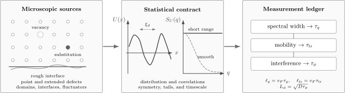
Disorder must be specified from source to statistic to observable. Point and extended defects generate a random field with a correlation length $\xi_d$ and power spectrum $S_U(q)$. Spectral broadening, momentum relaxation, and interference then probe $\tau_q$, $\tau_{\mathrm{tr}}$, and $\tau_\phi$; those times are not interchangeable.

The Statistical Contract

Mean and two-point correlation

For statistically homogeneous scalar disorder, write

$$\overline{U(\mathbf r)} = U_0,$$ $$C(\mathbf r-\mathbf r') = \overline{ \delta U(\mathbf r)\delta U(\mathbf r') }, \qquad \delta U=U-U_0.$$

The variance $C(\mathbf 0)$ measures amplitude, while the decay of $C(\mathbf r)$ defines one or more correlation lengths. “Disorder strength $W$” is incomplete unless the distribution and convention for $W$ are given.

Use the Fourier convention

$$U_{\mathbf q} = \int d^dr\, e^{-i\mathbf q\cdot\mathbf r} \delta U(\mathbf r).$$

Statistical homogeneity implies

$$\overline{ U_{\mathbf q}U_{\mathbf q'} } = (2\pi)^d \delta^{(d)}(\mathbf q+\mathbf q') S_U(\mathbf q),$$

where $S_U(\mathbf q)$ is the disorder power spectrum. Scattering from $\mathbf k$ to $\mathbf k'$ samples

$$\mathbf q = \mathbf k'-\mathbf k.$$

Short-range disorder has appreciable weight over large $q$ and can efficiently reverse momentum. Smooth disorder concentrates weight near $q=0$ and often causes many small-angle deflections before momentum is randomized.

White noise and correlated disorder

An idealized white-noise model is

$$C(\mathbf r-\mathbf r') = \gamma\, \delta^{(d)}(\mathbf r-\mathbf r').$$

Because of the delta function, $\gamma$ has units of energy squared times length to the power $d$ for a potential-energy field. White noise has no microscopic ultraviolet cutoff. A lattice spacing, impurity size, or finite correlation length must regularize predictions sensitive to short distances.

If $U$ is Gaussian, its mean and covariance determine all moments. If it is not Gaussian, higher cumulants, tails, and rare regions contain independent information. Two distributions with the same variance can have very different probabilities for a strong local defect.

Symmetry of the ensemble

An ensemble may preserve a symmetry statistically even though every realization breaks it. For example,

$$\overline{U(\mathbf r)} = 0$$

does not make one sample translation invariant. Restoring a symmetry after averaging does not restore Bloch momentum as an exact quantum number of that sample.

Time-reversal, spin-rotation, particle–hole, chiral, and crystalline symmetries constrain interference and topology. The disorder model must state whether the random term preserves each symmetry realization by realization, only in distribution, or not at all.

Scattering Times and Mean Free Paths

Quantum lifetime

For dilute, uncorrelated impurities and weak elastic scattering, Fermi’s golden rule gives the single-particle or quantum scattering rate

$$\frac{1}{\tau_q(\mathbf k)} = \frac{2\pi}{\hbar} n_i \int \frac{d^dk'}{(2\pi)^d} \lvert u_{\mathbf k'-\mathbf k}\rvert^2 \delta( \epsilon_{\mathbf k'} - \epsilon_{\mathbf k} ).$$

Every scattering event contributes, including a small-angle event that barely changes the current. This rate controls spectral broadening in the simplest weak-disorder picture.

For a disorder-averaged retarded Green function,

$$\overline{G^R(\mathbf k,E)} = \frac{1} {E-\epsilon_{\mathbf k}-\Sigma^R(\mathbf k,E)},$$

a weak, nearly energy-independent elastic rate is represented by

$$\operatorname{Im}\Sigma^R \simeq - \frac{\hbar}{2\tau_q}.$$

The corresponding Lorentzian spectral peak has full width at half maximum approximately $\hbar/\tau_q$. Interactions, instrumental resolution, inhomogeneous broadening, and energy-dependent self-energies can invalidate that direct identification.

Transport lifetime

For an isotropic band, the transport rate adds an angular weight:

$$\frac{1}{\tau_{\mathrm{tr}}(\mathbf k)} = \frac{2\pi}{\hbar} n_i \int \frac{d^dk'}{(2\pi)^d} \lvert u_{\mathbf k'-\mathbf k}\rvert^2 (1-\cos\theta) \delta( \epsilon_{\mathbf k'} - \epsilon_{\mathbf k} ).$$

Forward scattering has $\theta\approx0$ and contributes little to momentum relaxation. Therefore smooth disorder often gives

$$\tau_{\mathrm{tr}} \gg \tau_q.$$

For isotropic point scattering, the two can be comparable. In an anisotropic or multiband material, the simple $1-\cos\theta$ factor must be replaced by the appropriate velocity and band-overlap structure.

The associated lengths at the Fermi surface are

$$\ell_q = v_F\tau_q, \qquad \ell_{\mathrm{tr}} = v_F\tau_{\mathrm{tr}}.$$

Calling either quantity “the mean free path” without saying how it was inferred creates ambiguity.

Elastic scattering is not dephasing

A fixed random potential produces unitary evolution. It mixes momenta and makes paths complicated, but it does not by itself erase phase information in one isolated realization. The phase-coherence length

$$L_\phi = \sqrt{D\tau_\phi}$$

contains an inelastic or phase-randomizing time $\tau_\phi$. For isotropic diffusion in $d$ dimensions,

$$D = \frac{v_F^2\tau_{\mathrm{tr}}}{d}.$$

The regimes

$$L \ll \ell_{\mathrm{tr}}$$

and

$$\ell_{\mathrm{tr}} \ll L$$

are respectively ballistic and diffusive at the sample scale $L$. If the diffusive sample also has $L\lesssim L_\phi$, coherent multiple scattering produces mesoscopic interference. Quantum Coherence in Conductors owns the dephasing ledger.

Weak-disorder parameter

For a Fermi liquid with well-defined $k_F$, the dimensionless product

$$k_F\ell_{\mathrm{tr}}$$

is a common disorder diagnostic. Semiclassical transport is controlled when it is large. The regime $k_F\ell\sim1$ is often called the Mott–Ioffe–Regel crossover, where a wavelength and mean free path are no longer well separated.

This is a warning criterion, not a universal theorem locating a metal–insulator transition. Strong correlations, multiband structure, anisotropy, and the choice of lifetime can make a naive $k_F\ell$ estimate misleading.

What a Disorder Average Does

Average observables, not a fictitious crystal

For an observable $X[U]$, one may seek

$$\overline{X} = \int\mathcal DU\, P[U]X[U].$$

Replacing $U$ by its mean before solving usually loses scattering:

$$X[\overline U] \neq \overline{X[U]}.$$

The coherent-potential approximation, self-consistent Born approximation, replica method, supersymmetry, and numerical ensemble averaging are different ways to address this nonlinearity. Each preserves different information and has different failure modes.

An averaged one-particle Green function can describe a mean density of states and linewidth, but conductivity involves products of Green functions and vertex corrections. A single self-energy is not automatically a transport theory.

Self-averaging and mesoscopic fluctuations

An extensive observable built from many weakly correlated regions may become self-averaging:

$$\frac{\operatorname{Var}X} {\overline X^{\,2}} \longrightarrow 0$$

as sample volume grows. This limit is not automatic near a critical point, with long-range-correlated disorder, or for observables dominated by rare regions.

Mesoscopic conductance is explicitly sample-specific. Repeating a magnetic-field sweep on one coherent device can reveal a reproducible fluctuation pattern, while averaging many samples or a broad energy interval suppresses it. Universal Conductance Fluctuations is the canonical home for that distinction.

What counts as an ensemble experimentally

An experimental disorder average may use:

• many nominally identical samples;
• different regions of one large sample;
• repeated impurity configurations after thermal cycling;
• energy, gate-voltage, or magnetic-field windows under an ergodic assumption; or
• time averaging if the disorder itself moves.

These procedures are not interchangeable. Field sweeping changes interference phases without necessarily changing the defects. Thermal cycling may change both disorder and contact conditions. A paper should identify the ensemble actually sampled.

Disorder as a Tuning Parameter

Disorder can destroy clean behavior, reveal hidden scales, or create a useful regime.

Carrier density and randomness can be entangled

Chemical substitution often changes both the carrier concentration and the random potential. A phase diagram plotted against dopant fraction therefore mixes at least two control axes. Gating, pressure, isovalent substitution, and irradiation can help separate them, but each introduces its own secondary changes.

A causal disorder study should compare samples at matched density where possible and report structural, spectral, and transport diagnostics rather than using composition alone.

Order and superconductivity

Random fields can pin density waves and domains. Random masses can broaden a transition. Rare regions can retain local order beyond the clean transition. The outcome depends on dimensionality, symmetry, correlation length, and whether disorder couples to the order parameter directly.

For an isotropic conventional $s$-wave superconductor, nonmagnetic elastic disorder does not strongly suppress $T_c$ under the assumptions of Anderson’s theorem. Magnetic scattering, unconventional gap structure, strong inhomogeneity, and proximity to localization fall outside that simple protection. BCS Theory owns the clean pairing framework.

Topology and quantized response

Moderate symmetry-preserving disorder can leave a topological phase intact as long as the relevant mobility or spectral gap remains effective. In the integer quantum Hall effect, localized bulk states help produce a finite interval of filling over which the Hall response remains quantized.

Some model Hamiltonians exhibit disorder-driven topological phases. Calling a material a “topological Anderson insulator” requires more than an increasing resistance or an edge-like signal: one needs a disorder-aware invariant or mobility-gap analysis, bulk and boundary evidence, and controls against ordinary inhomogeneous conduction.

Disorder engineering

Controlled irradiation, alloying, patterned vacancies, correlated roughness, and quasiperiodic potentials can be experimental knobs. “More disorder” is still inadequate. The intervention should be tied to a measured defect density, correlation function, symmetry change, or scattering spectrum.

Measurement Ledger

Observable	Most direct sensitivity	Frequent trap
residual resistivity or mobility	momentum-relaxing rate and carrier parameters	attributing every change to defect density in a multiband material
quantum-oscillation Dingle factor	quantum lifetime and orbit-dependent broadening	equating $\tau_q$ with $\tau_{\mathrm{tr}}$
ARPES linewidth	single-particle self-energy plus resolution	assigning interaction and disorder broadening uniquely from one spectrum
STM or STS map	local density of states and defect resonances	reading the local density of states as the bare random potential
diffuse x-ray or neutron scattering	structural correlations away from Bragg peaks	missing electronically active defects with weak structural contrast
electron microscopy	local composition and extended defects	generalizing a small field of view to a whole transport device
low-frequency noise	dynamic fluctuators and switching-rate distribution	using dynamic noise as a complete measure of quenched disorder
sample-to-sample statistics	yield, tails, and parameter correlations	publishing only selected functional devices

No single probe reconstructs $P[U]$. A trustworthy disorder model is triangulated from structure, spectroscopy, transport, and statistics.

Common Mistakes

• Treating static disorder as decoherence. Elastic scattering preserves phase in a fixed realization.
• Quoting one “mean free path.” State whether it comes from spectral, quantum-oscillation, or transport data.
• Replacing the random field by its mean. Scattering and localization depend on fluctuations and correlations.
• Specifying only a variance. Correlation length, distribution tails, symmetry, and dynamics can change the physics.
• Assuming disorder averaging restores a clean sample. Statistical symmetry is not exact symmetry of one realization.
• Using $k_F\ell\sim1$ as an exact phase boundary. It is a regime diagnostic with model-dependent meaning.
• Changing dopant concentration and calling the result a pure disorder sweep. Density, strain, chemistry, and interactions may change too.
• Inferring a bare defect potential from one measured image. Every probe has a response function and finite resolution.

Exercises

1. Binary-alloy statistics

At each lattice site, let $\epsilon_i=V_A$ with probability $p$ and $\epsilon_i=V_B$ with probability $1-p$. Find the mean and variance.

Solution

The mean is

$$\overline{\epsilon} = pV_A+(1-p)V_B.$$

Using either direct expansion or the two-point distribution,

$$\begin{aligned} \operatorname{Var}\epsilon &= p(V_A-\overline\epsilon)^2 + (1-p)(V_B-\overline\epsilon)^2 \\ &= p(1-p)(V_A-V_B)^2. \end{aligned}$$

The variance vanishes for a pure crystal, $p=0$ or $1$, and is largest at $p=1/2$ for fixed $V_A-V_B$.

2. Gaussian-correlated disorder

For

$$C(\mathbf r) = W^2 \exp\!\left( - \frac{r^2}{2\xi_d^2} \right),$$

find the power spectrum $S_U(\mathbf q)$ in $d$ dimensions using the Fourier convention on this page.

Solution

The Fourier transform of a $d$-dimensional Gaussian factorizes:

$$S_U(\mathbf q) = \int d^dr\, e^{-i\mathbf q\cdot\mathbf r} C(\mathbf r).$$

Therefore

$$S_U(\mathbf q) = (2\pi)^{d/2} W^2\xi_d^d \exp\!\left( - \frac{q^2\xi_d^2}{2} \right).$$

Large $\xi_d$ narrows the spectrum around $q=0$, suppressing large-momentum-transfer scattering.

3. Disorder is not automatically decoherence

An electron evolves under one time-independent random Hamiltonian $H_U$. Show that purity is conserved. Why can an ensemble-averaged density matrix nevertheless lose purity?

Solution

For one realization,

$$\rho_U(t) = e^{-iH_Ut/\hbar} \rho(0) e^{iH_Ut/\hbar}.$$

Unitary conjugation preserves

$$\operatorname{Tr}\rho_U(t)^2 = \operatorname{Tr}\rho(0)^2.$$

If realizations are not recorded, the ensemble state is

$$\overline\rho(t) = \int\mathcal DU\, P[U]\rho_U(t).$$

A mixture of differently rotated pure states can have

$$\operatorname{Tr}\overline\rho(t)^2<1.$$

This is ensemble dephasing from missing classical information, not microscopic nonunitarity within any realization. Dynamic disorder or an uncontrolled environment can produce genuine open-system decoherence.

4. Quantum and transport lifetimes

In two dimensions, suppose the angular scattering weight on the Fermi circle is

$$W(\theta) = W_0(1+a\cos\theta), \qquad \lvert a\rvert<1.$$

Find $\tau_{\mathrm{tr}}/\tau_q$.

Solution

Ignoring their common prefactor,

$$\frac{1}{\tau_q} \propto \int_0^{2\pi} W(\theta)\,d\theta = 2\pi W_0.$$

For transport,

$$\begin{aligned} \frac{1}{\tau_{\mathrm{tr}}} &\propto \int_0^{2\pi} W(\theta)(1-\cos\theta)\,d\theta \\ &= \pi W_0(2-a). \end{aligned}$$

Hence

$$\frac{\tau_{\mathrm{tr}}}{\tau_q} = \frac{2}{2-a}.$$

Positive $a$ favors forward scattering and gives $\tau_{\mathrm{tr}}>\tau_q$. For $a=0.8$, the ratio is $5/3$.

5. Mean free path from mobility

A spin-degenerate two-dimensional electron gas has density

$$n = 3.0\times10^{11}\,\mathrm{cm}^{-2}$$

and mobility

$$\mu = 1.0\times10^6\,\mathrm{cm}^2/(\mathrm{V\,s}).$$

Assuming one circular parabolic band, estimate $k_F$, $\ell_{\mathrm{tr}}$, and $k_F\ell_{\mathrm{tr}}$.

Solution

Convert units:

$$n = 3.0\times10^{15}\,\mathrm{m}^{-2}, \qquad \mu = 100\,\mathrm{m}^2/(\mathrm{V\,s}).$$

For spin degeneracy two,

$$k_F = \sqrt{2\pi n} \approx 1.37\times10^8\,\mathrm{m}^{-1}.$$

Using $\mu=e\tau_{\mathrm{tr}}/m^*$ and $v_F=\hbar k_F/m^*$,

$$\ell_{\mathrm{tr}} = v_F\tau_{\mathrm{tr}} = \frac{\hbar k_F\mu}{e}.$$

Numerically,

$$\ell_{\mathrm{tr}} \approx 9.0\,\mu\mathrm m,$$

and

$$k_F\ell_{\mathrm{tr}} \approx 1.24\times10^3.$$

The effective mass cancels in this ideal one-band estimate. Multiband conduction, density-dependent scattering, or an incorrect degeneracy would change the inference.

6. Self-energy and linewidth

A weak-disorder retarded self-energy has

$$\Sigma^R = \Delta E - i\frac{\hbar}{2\tau_q}.$$

Show that the corresponding spectral peak has full width at half maximum $\hbar/\tau_q$.

Solution

Near the renormalized pole $E_0=\epsilon_{\mathbf k}+\Delta E$,

$$G^R(E) = \frac{1} {E-E_0+i\hbar/(2\tau_q)}.$$

The spectral function is proportional to

$$A(E) \propto \frac{\hbar/(2\tau_q)} {(E-E_0)^2+[\hbar/(2\tau_q)]^2}.$$

Its half width at half maximum is $\hbar/(2\tau_q)$, so the full width is

$$\mathrm{FWHM} = \frac{\hbar}{\tau_q}.$$

This extraction assumes a Lorentzian line, weak energy dependence of the self-energy, and separately controlled instrumental broadening.

7. Quenched versus annealed free energy

Use Jensen’s inequality to compare $F_{\mathrm q}$ and $F_{\mathrm a}$.

Solution

Because $\ln x$ is concave,

$$\overline{\ln Z_U} \le \ln\overline{Z_U}.$$

Multiplication by $-k_BT$ reverses the inequality:

$$F_{\mathrm q} \ge F_{\mathrm a}.$$

The annealed system can lower its free energy by redistributing the disorder variables together with the matter degrees of freedom. Frozen disorder lacks that equilibration channel.

8. Audit a disorder-driven transition

A material becomes insulating as substitution $x$ increases. The authors attribute the transition to Anderson localization because the residual resistivity rises. List at least six additional checks.

Solution

A convincing analysis should examine:

• carrier density and Fermi-surface changes with $x$;
• structural phases, strain, and possible percolation;
• interaction-driven gaps or magnetic ordering;
• the temperature dependence and scaling of conductivity;
• localization-length or mobility-edge evidence where accessible;
• quantum versus transport lifetimes;
• spatial inhomogeneity and rare conducting paths;
• sample-to-sample statistics and contact effects;
• controlled disorder at approximately fixed filling; and
• spectroscopy for a band gap, pseudogap, or spectral-weight transfer.

Rising residual resistivity establishes stronger momentum relaxation. It does not uniquely identify a localization mechanism or exclude a Mott, band, magnetic, structural, or granular transition.

Connections

• Conventions for Quantum Matter fixes Fourier, charge, current, and spectral conventions used here.
• Device Fabrication Concepts maps residues, etch damage, traps, roughness, strain, contact reactions, and thermal mismatch onto process controls and device distributions.
• Data Interpretation and Pitfalls shows how disorder distributions, phase fractions, and connectivity can imitate or obscure a homogeneous intrinsic response.
• First Born Approximation derives weak-potential scattering amplitudes and validity conditions.
• Fermi’s Golden Rule owns the general transition-rate derivation.
• Drude Theory connects a transport relaxation time to conductivity and optical response.
• Boltzmann Transport develops the collision operator, anisotropic scattering, and state-resolved distribution.
• Spectral Functions owns the relation among poles, widths, quasiparticle weight, and measured spectra.
• Quantum Coherence in Conductors separates elastic scattering, escape, thermal averaging, and dephasing.
• Weak Localization turns those elastic and coherence scales into the leading interference correction and its low-field magnetoconductance.
• Universal Conductance Fluctuations develops sample-specific coherent fluctuations and ensemble logic.
• Anderson Localization takes the declared disorder ensemble into the strong-interference regime of localized eigenstates, bounded spreading, and exponentially small typical transmission.
• Scaling Theory of Localization follows the dimensionless conductance from the mean-free-path scale toward metallic, localized, or critical infrared behavior.
• Anderson Insulators separates zero-temperature localization from bath-assisted hopping and interaction-induced Coulomb-gap transport.
• Mobility Edges maps the energy–disorder boundary between localized and extended states and audits its finite-size and experimental resolution.
• Random Matrix Theory in Quantum Matter supplies symmetry-resolved spectral benchmarks for metallic, localized, and critical regimes.
• Glasses and Spin Glasses develops the distinct case in which quenched randomness and frustration produce overlap order, collective freezing, and aging.
• One-over-f Noise treats broad ensembles of dynamic fluctuators.
• BCS Theory supplies the clean pairing state needed to state disorder robustness and pair-breaking limits.
• Superconducting Proximity Effect takes the disorder ensemble and elastic scales declared here into dirty-limit validity tests, inverse proximity, pair breaking, and self-consistent spatial correlations.
• Vortex Matter, Pinning, and Flux Flow owns how declared defects and disorder landscapes become vortex pinning, collective creep, critical states, and driven mixed-state response.
• Integer Quantum Hall Effect shows how localized bulk states support plateau intervals around quantized Hall response.

References

1. P. W. Anderson, “Absence of Diffusion in Certain Random Lattices,” Physical Review 109, 1492–1505 (1958), doi:10.1103/PhysRev.109.1492.
2. P. W. Anderson, “Theory of Dirty Superconductors,” Journal of Physics and Chemistry of Solids 11, 26–30 (1959), doi:10.1016/0022-3697(59)90036-8.
3. P. Soven, “Coherent-Potential Model of Substitutional Disordered Alloys,” Physical Review 156, 809–813 (1967), doi:10.1103/PhysRev.156.809.
4. R. J. Elliott, J. A. Krumhansl, and P. L. Leath, “The Theory and Properties of Randomly Disordered Crystals and Related Physical Systems,” Reviews of Modern Physics 46, 465–543 (1974), doi:10.1103/RevModPhys.46.465.
5. E. Abrahams, P. W. Anderson, D. C. Licciardello, and T. V. Ramakrishnan, “Scaling Theory of Localization: Absence of Quantum Diffusion in Two Dimensions,” Physical Review Letters 42, 673–676 (1979), doi:10.1103/PhysRevLett.42.673.
6. P. A. Lee and T. V. Ramakrishnan, “Disordered Electronic Systems,” Reviews of Modern Physics 57, 287–337 (1985), doi:10.1103/RevModPhys.57.287.
7. F. Evers and A. D. Mirlin, “Anderson Transitions,” Reviews of Modern Physics 80, 1355–1417 (2008), doi:10.1103/RevModPhys.80.1355.
8. N. E. Hussey, K. Takenaka, and H. Takagi, “Universality of the Mott–Ioffe–Regel Limit in Metals,” Philosophical Magazine 84, 2847–2864 (2004), doi:10.1080/14786430410001716944.
9. A. Lagendijk, B. van Tiggelen, and D. S. Wiersma, “Fifty Years of Anderson Localization,” Physics Today 62(8), 24–29 (2009), doi:10.1063/1.3206091.
10. J. M. Ziman, Models of Disorder: The Theoretical Physics of Homogeneously Disordered Systems, Cambridge University Press, 1979.
11. E. N. Economou, Green’s Functions in Quantum Physics, 3rd ed., Springer, 2006, doi:10.1007/3-540-28841-4.
12. E. Akkermans and G. Montambaux, Mesoscopic Physics of Electrons and Photons, Cambridge University Press, 2007, doi:10.1017/CBO9780511618833.
13. H. Bruus and K. Flensberg, Many-Body Quantum Theory in Condensed Matter Physics, Oxford University Press, 2004, doi:10.1093/acprof:oso/9780198566335.001.0001.
14. S. Datta, Electronic Transport in Mesoscopic Systems, Cambridge University Press, 1995, doi:10.1017/CBO9780511805776.
15. J. Rammer, Quantum Field Theory of Non-equilibrium States, Cambridge University Press, 2007, doi:10.1017/CBO9780511618956.

Further reading

• A. Altland and B. Simons, Condensed Matter Field Theory, 2nd ed., Cambridge University Press, 2010. See the disorder, replica, nonlinear-sigma-model, and localization chapters.
• N. F. Mott and E. A. Davis, Electronic Processes in Non-Crystalline Materials, 2nd ed., Oxford University Press, 1979.