Open Quantum Materials

An open quantum material is a many-body material or synthetic-matter platform whose relevant states, spectra, or functions depend essentially on coupling to degrees of freedom outside the retained model. Those degrees of freedom may be phonons, photons, substrates, electrical leads, defects, fluctuating fields, measurement channels, or deliberately engineered reservoirs. “Open” is a modeling boundary, not a new chemical category: the same sample can be treated as closed for a femtosecond coherent process and open for transport, relaxation, or steady-state preparation.

This page owns the materials-facing hierarchy from microscopic environments to complex quasiparticle poles, dissipative state design, non-Hermitian band models, and exceptional-point evidence. System–Bath Hamiltonians owns the generic microscopic decomposition. Reservoir Engineering owns the general control design. Quantum-Jump Simulation owns trajectory algorithms. Feshbach Projection Formalism owns the full energy-dependent projection derivation. Driven-Dissipative Matter owns sustained pump–loss phases and polariton transition evidence.

Materials Coupled to Environments

A useful microscopic starting point is

$$H_{\mathrm{tot}} = H_M + H_E + \sum_\alpha A_\alpha\otimes B_\alpha.$$

$H_M$ contains the material degrees of freedom retained in the calculation, $H_E$ contains the environment, and $A_\alpha\otimes B_\alpha$ specifies what the environment can monitor or exchange. The split must be declared. Treating a cavity photon, optical phonon, or metallic lead as part of $M$ in one model and tracing it into $E$ in another changes both the state space and the observables.

Common material environments include:

• acoustic and optical phonons that exchange energy and momentum;
• electromagnetic vacuum, cavities, waveguides, and radiative continua;
• substrates, gates, adsorbates, and fluctuating charges;
• metallic leads and particle reservoirs;
• magnons, nuclear spins, and other slow internal sectors;
• disorder configurations that may be static, slowly fluctuating, or annealed;
• pump and probe fields, detectors, and feedback electronics.

Calling all these influences “decoherence” loses important distinctions. A bath can shift levels, broaden poles, thermalize occupations, dephase selected coherences, remove particles, mediate interactions, or create correlated noise. Phonons can destroy electronic phase coherence and also mediate pairing. A cavity can provide loss and also reorganize collective modes. The sign and usefulness of an environmental effect are questions about a specified observable and timescale.

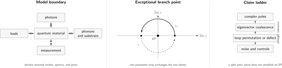
Open-material reasoning proceeds in three stages: declare the retained boundary, identify the complex spectral or dynamical singularity, and match the claim to an evidence ladder. An exceptional point requires coalescing eigenvectors or equivalent branch evidence, not merely two unresolved peaks.

Environment ledger

Before choosing a reduced model, record:

Layer	Questions
boundary	Which electrons, spins, photons, phonons, leads, and detectors are retained?
coupling	Which operators $A_\alpha$ and $B_\alpha$ exchange energy, particles, or phase information?
spectrum	Is the bath smooth, gapped, resonant, thermal, squeezed, driven, or spatially structured?
clocks	How do bath memory, relaxation, drive, traversal, and measurement times compare?
state	Is the environment thermal, stationary nonequilibrium, correlated, or initially entangled with the material?
observable	Is the experiment measuring a density matrix, spectral pole, scattering amplitude, current, or conditioned record?

The bath correlation matrix

$$S_{\alpha\beta}(\omega) = \int_{-\infty}^{\infty} dt\, e^{i\omega t} \left\langle B_\alpha(t)B_\beta(0) \right\rangle_E$$

helps determine transition rates and noise. A Markov approximation requires more than weak coupling: the relevant environmental correlations must decay rapidly compared with the retained evolution, and the system frequencies sampled by the coupling must be resolved consistently. Near a band edge, sharp phonon resonance, cavity pole, or critical environment, memory can be the leading physics.

Choosing a Reduced Description

No single “open Hamiltonian” contains every open-system observable. Different reductions preserve different information.

Target	Useful description	What it retains
populations and coherences	reduced density matrix or master equation	trace, positivity, mixed states, jump channels
quasiparticle energies and lifetimes	retarded Green function and self-energy	complex poles and spectral weight
transport through leads	nonequilibrium Green functions or scattering matrix	currents, contacts, occupations, channel amplitudes
conditioned detection record	quantum trajectories	no-click evolution and stochastic jumps
collective response and noise	Schwinger–Keldysh field theory	response, correlations, memory, and coarse-grained fields
resonances in a retained subspace	Feshbach or optical-potential reduction	energy-dependent shifts, widths, and outgoing poles

Agreement between two descriptions is conditional. A Lindblad equation can imply a retarded response, but its jump operators contain information that an effective non-Hermitian Hamiltonian alone omits. A retarded self-energy gives linewidths but does not by itself fix occupations; the Keldysh or lesser component carries distribution information.

Self-energy and spectral weight

For a translationally organized material, a retarded single-particle Green function can be written

$$G^R(\mathbf k,\omega) = \left[ \left( \hbar\omega+i0^+ \right)I - H_0(\mathbf k) - \Sigma^R(\mathbf k,\omega) \right]^{-1}.$$

The spectral function is

$$\mathcal A(\mathbf k,\omega) = -\frac{1}{\pi} \operatorname{Im} \operatorname{Tr} G^R(\mathbf k,\omega).$$

The Hermitian part of $\Sigma^R$ shifts and mixes quasiparticle levels. Its anti-Hermitian part gives finite lifetime and can mix decay channels. Both may depend strongly on frequency and momentum. Replacing $\Sigma^R(\omega)$ by a constant matrix is controlled only over a declared spectral window.

A complex pole

$$z_n = \varepsilon_n - \frac{i}{2}\Gamma_n$$

has a decay width $\Gamma_n>0$ under the convention $e^{-iz_nt/\hbar}$. The measured spectral peak need not sit exactly at $\operatorname{Re}z_n$ when backgrounds, overlapping resonances, matrix elements, or frequency-dependent self-energies distort the line shape.

Dissipation as a Design Tool

Environmental coupling becomes a design tool when its spectrum, geometry, or monitored channel is deliberately chosen to stabilize a useful state or response. Examples include cooling selected modes, optically pumping a spin sector, making an entangled state dark, removing defects faster than they are created, or engineering a topological steady-state covariance matrix.

In a Markovian model,

$$\dot\rho = -\frac{i}{\hbar} [H,\rho] + \sum_\mu \mathcal D[L_\mu]\rho.$$

The target $\rho_\star$ must satisfy

$$\mathcal L\rho_\star=0,$$

but stationarity is only the first test. A material-scale preparation proposal must also establish:

1. Attractivity. Unwanted states flow toward the target rather than into other dark sectors.
2. Rate. The dissipative gap remains large enough for preparation before natural errors act.
3. Locality. The proposed jump processes can be implemented with available couplings and geometry.
4. Scalability. Preparation time and error do not become impractical with system size.
5. Verification. Accessible observables distinguish the target from nearby mixed states.
6. Thermodynamics. Pump power, entropy export, and auxiliary reset costs are included.

In a simple perturbative error regime, one often expects

$$1-F_\star \sim \frac{ \Gamma_{\mathrm{bad}} }{ \Delta_{\mathcal L} },$$

where $\Gamma_{\mathrm{bad}}$ summarizes harmful channels and $\Delta_{\mathcal L}$ is a useful relaxation scale. This is a scaling estimate, not a theorem. Nonnormality, degeneracy, diffusion, and correlated errors can alter it.

Engineered dissipation has rigorous and constructive successes, including entangled-state preparation and proposed topological steady states. It is not automatically faster than cooling. A 2026 comparison of passive and engineered topological preparation found diffusion-limited quadratic growth of preparation time with linear system size in the protocols studied. The correct claim is therefore platform and scaling specific: dissipation can create a target that coherent ground-state cooling does not easily reach, while still facing locality and transport bottlenecks.

Non-Hermitian Effective Hamiltonians

A non-Hermitian Hamiltonian is usually an effective generator, pole equation, or wave operator. Its physical meaning depends on how it was obtained.

Conditional no-jump evolution

For a monitored Lindblad model, the unnormalized state between detected jumps evolves with

$$H_{\mathrm{eff}} = H - \frac{i\hbar}{2} \sum_\mu L_\mu^\dagger L_\mu.$$

Its norm obeys

$$\frac{d}{dt} \langle\tilde\psi\vert\tilde\psi\rangle = - \sum_\mu \left\langle L_\mu^\dagger L_\mu \right\rangle_{\tilde\psi}.$$

The lost norm is survival probability for a specified monitoring record. It is not destruction of total probability in the unconditional experiment. Restoring the jumps and averaging records recovers trace-preserving density-matrix evolution. The choice of unraveling also depends on what is monitored; photon counting, homodyne detection, and unobserved loss do not define the same conditional pure-state process.

Projection and resonance poles

Let $P$ retain a material subspace and $Q=I-P$ contain eliminated states. Outgoing boundary conditions give an energy-dependent operator

$$\begin{aligned} H_{\mathrm{eff}}(E) ={}& PHP \\ &+ PHQ \frac{1}{ E-QHQ+i0^+ } QHP. \end{aligned}$$

The second term is a self-energy. Above an open threshold it acquires an anti-Hermitian part. Resonance poles solve

$$\det\!\left[ E-H_{\mathrm{eff}}(E) \right] = 0,$$

so diagonalizing a frozen matrix at one real $E$ can miss energy dependence, extra roots, and threshold structure. Feshbach Projection Formalism develops the state reconstruction and normalization that accompany this reduction.

Phenomenological mode and band models

Classical photonic, acoustic, mechanical, and circuit platforms often produce a non-Hermitian eigenproblem directly after imposing radiation, absorption, gain, or impedance boundary conditions. Electronic quasiparticle models can instead use

$$H_{\mathrm{qp}}(\mathbf k,\omega) = H_0(\mathbf k) + \Sigma^R(\mathbf k,\omega).$$

The microscopic many-body Hamiltonian may remain Hermitian even though the quasiparticle pole operator is not. Complex bands then organize frequency and lifetime, but they are not a list of stationary energies of an isolated crystal.

Left and right eigenvectors

For a diagonalizable non-Hermitian matrix,

$$\begin{aligned} H_{\mathrm{eff}} \lvert R_n\rangle &= z_n\lvert R_n\rangle, \\ \langle L_n\rvert H_{\mathrm{eff}} &= z_n\langle L_n\rvert. \end{aligned}$$

The left and right vectors can be normalized biorthogonally:

$$\langle L_m\vert R_n\rangle = \delta_{mn}.$$

Right eigenvectors alone need not be orthogonal, and the matrix can be highly nonnormal. Small perturbations can then produce large eigenvector and transient-response changes even away from an exact degeneracy.

The biorthogonal quantity $\langle L_n\vert O\vert R_n\rangle$ is mathematically natural, but it is not automatically a laboratory expectation value. Physical observables must be derived from the underlying density matrix, Green function, scattering state, or measurement protocol. This distinction prevents the effective eigenproblem from silently replacing the open-system experiment.

Exceptional Points in Matter

An exceptional point is a parameter value at which eigenvalues and their eigenvectors coalesce, making the effective operator defective. It differs from a Hermitian diabolic point, where degenerate eigenvectors can remain linearly independent and orthogonal.

Two-mode model

Consider two reciprocal modes with complex bare frequencies

$$\Omega_j = \omega_j - \frac{i}{2}\gamma_j$$

and real coupling $g$:

$$H_2 = \begin{pmatrix} \Omega_1 & g \\ g & \Omega_2 \end{pmatrix}.$$

The eigenvalues are

$$z_\pm = \frac{\Omega_1+\Omega_2}{2} \pm \sqrt{ g^2 + \left( \frac{\Omega_1-\Omega_2}{2} \right)^2 }.$$

The exceptional-point condition is the vanishing of the discriminant,

$$g^2 + \left( \frac{\Omega_1-\Omega_2}{2} \right)^2 = 0.$$

If $\omega_1=\omega_2$ and $g$ is real, this reduces to

$$g = \frac{ \lvert\gamma_1-\gamma_2\rvert }{4}.$$

At that point, the two eigenvalues share one eigenvector. Near a generic second-order exceptional point, a perturbation $\epsilon$ produces

$$z_+-z_- \propto \sqrt{\epsilon}.$$

Because the discriminant is complex, two real conditions generally have to be satisfied. A generic second-order exceptional point therefore has codimension two unless a symmetry or constraint reduces the tuning requirement.

Branch topology and encircling

The square root gives two sheets. Encircling the exceptional point once in a two-parameter plane exchanges $z_+$ and $z_-$. A second loop returns the eigenvalue branch, possibly with an additional geometric phase depending on convention and path.

Static analytic continuation and dynamical encircling must be separated. In a lossy system, arbitrarily slow evolution need not follow an instantaneous eigenstate: differential decay and Stokes transitions can select one mode and produce direction-dependent transfer. Experiments by Doppler and collaborators and by Xu and collaborators demonstrated asymmetric mode conversion in microwave and optomechanical settings. Their dynamical outcomes contain the exceptional-point topology together with nonadiabatic open-system evolution.

Exceptional points from material lifetimes

Interactions and disorder give orbital-dependent self-energies. When two quasiparticle sectors have different lifetimes, the anti-Hermitian part of the self-energy can turn an ordinary band crossing into exceptional points connected by a locus where the real parts of the poles coincide. Kozii and Fu developed this finite-lifetime quasiparticle mechanism; dynamical mean-field calculations by Nagai and collaborators found corresponding bulk-arc structures in heavy-fermion models.

The inference remains spectral and model dependent. An intensity ridge that resembles an arc is not sufficient. One should reconstruct complex poles or a controlled self-energy, verify the defective points at the arc ends, and exclude matrix-element zeros, surface states, finite resolution, and ordinary lifetime-broadened crossings.

Boundaries and the skin effect

Non-Hermitian lattice spectra can depend strongly on boundary conditions. Under the non-Hermitian skin effect, an extensive number of right eigenmodes accumulate near a boundary, so periodic Bloch bands may fail to predict an open sample. A point-gap winding in one dimension can be defined by

$$\nu(E_0) = \frac{1}{2\pi i} \int_{\mathrm{BZ}} dk\, \partial_k \log\det\!\left[ H(k)-E_0 \right].$$

This invariant is meaningful only when the reference point $E_0$ lies outside the periodic complex spectrum. Open-boundary predictions may require a generalized, non-Bloch Brillouin zone. Boundary localization in a pumped or lossy experiment must also be distinguished from ordinary attenuation, source placement, defects, and finite propagation length.

Experimental Cautions

A split peak is not an exceptional point

An avoided crossing in frequency, a crossing in linewidth, or a change in intensity can suggest a two-mode non-Hermitian model. Stronger evidence tracks both real and imaginary pole components and tests eigenvector behavior.

Claim level	Useful evidence
coupled lossy modes	calibrated complex response fitted across a parameter region
pole degeneracy	simultaneous coalescence of frequency and linewidth within uncertainty
exceptional point	eigenvector coalescence, defective response, or square-root branch structure
topological branch point	mode permutation or invariant around a closed two-parameter loop
material exceptional phase	momentum-resolved locus, endpoint defects, and boundary/geometry controls
device advantage	task-level signal-to-noise, bandwidth, stability, and resource comparison

Scattering poles and zeros are distinct. Coherent perfect absorption concerns a zero of a scattering eigenvalue; lasing concerns a pole reaching the real axis. Either can interact with exceptional structures, but neither is identical to an exceptional point.

Fit the complex response

Intensity-only spectra discard phase and can merge nearby modes. Whenever possible, measure a complex scattering amplitude, homodyne quadratures, time-domain ringdown, or interferometric field. Report:

• the instrument response and frequency calibration;
• background and Fano interference terms;
• gain saturation and pump-dependent heating;
• all fit parameters and uncertainty covariance;
• alternative two-pole and nondegenerate models;
• stability under fitting window and baseline choices.

Near a defective point, eigenvectors are ill conditioned. Parameter estimates can therefore have strongly correlated uncertainties, and a tiny residual can move the inferred exceptional point substantially.

Responsivity is not precision

The square-root splitting $\Delta z\propto\sqrt{\epsilon}$ gives large eigenvalue responsivity to a small perturbation. Metrological precision also depends on linewidth, noise, integration time, estimator bias, technical drift, and the resources needed to hold the device near the exceptional point.

Experiments have demonstrated enhanced splitting near exceptional points. Theory and noise measurements show that nonorthogonality can simultaneously increase excess noise, canceling the apparent advantage in reciprocal sensor classes. A trustworthy sensing comparison holds input power, bandwidth, integration time, detector efficiency, and prior calibration fixed, then reports uncertainty in the estimated perturbation rather than splitting alone.

Practical Workflow

1. Draw the boundary. State which material, bath, lead, cavity, and detector modes are retained.
2. Identify the observable. Density matrix, current, scattering pole, spectral function, or trajectory record.
3. Choose the reduction. Master equation, self-energy, scattering matrix, Keldysh action, or projection operator.
4. Derive non-Hermiticity. Show which loss, gain, continuum, or conditioning produces each anti-Hermitian term.
5. Test frequency and size dependence. Constant widths and local jumps need controlled windows.
6. Reconstruct complex information. Track frequencies, linewidths, phases, and eigenvectors where possible.
7. Compare boundaries. For lattices, test periodic, open, geometry, and source-location dependence.
8. Audit noise and resources. Convert enhanced response into task-level uncertainty or preparation fidelity.
9. Preserve the full model. Check key claims against the trace-preserving or microscopic description.

Common Mistakes

• Treating every real material as “non-Hermitian” without specifying the reduced operator.
• Using a constant imaginary potential across a spectral range where the self-energy varies strongly.
• Interpreting no-jump norm loss as unconditional loss of total probability.
• Computing physical expectation values from right eigenvectors with the ordinary inner product.
• Calling coincident real frequencies an exceptional point while linewidths remain distinct.
• Calling an avoided crossing or unresolved doublet an exceptional point without eigenvector evidence.
• Assuming slower encircling always improves adiabatic following.
• Applying periodic Bloch invariants directly to an open chain with a skin effect.
• Equating large eigenvalue splitting with improved parameter-estimation precision.
• Proposing engineered dissipation without a preparation-time, natural-error, and scalability audit.

Exercises

1. A Lorentzian pole

For

$$G^R(E) = \frac{1}{ E-\varepsilon+i\Gamma/2 },$$

derive the spectral function $A(E)=-(1/\pi)\operatorname{Im}G^R(E)$ and show that its integral over $E$ is one.

Solution

Multiplying by the complex conjugate denominator gives

$$G^R(E) = \frac{ E-\varepsilon-i\Gamma/2 }{ \left( E-\varepsilon \right)^2 + \left( \Gamma/2 \right)^2 }.$$

Therefore

$$A(E) = \frac{1}{\pi} \frac{ \Gamma/2 }{ \left( E-\varepsilon \right)^2 + \left( \Gamma/2 \right)^2 }.$$

Using $\int_{-\infty}^{\infty}dx\,a/(x^2+a^2)=\pi$ gives $\int dE\,A(E)=1$. Frequency-dependent self-energy or missing spectral sectors can change this simple normalization within a reduced window.

2. No-jump survival

A two-level emitter has $L=\sqrt{\gamma}\lvert g\rangle\langle e\rvert$ and $H=0$. Starting in $\lvert e\rangle$, find the unnormalized no-jump state and its norm.

Solution

Since

$$L^\dagger L = \gamma \lvert e\rangle\langle e\rvert,$$

the conditional generator is

$$H_{\mathrm{eff}} = -\frac{i\hbar\gamma}{2} \lvert e\rangle\langle e\rvert.$$

Thus

$$\lvert\tilde\psi(t)\rangle = e^{-\gamma t/2} \lvert e\rangle, \qquad \langle\tilde\psi(t)\vert\tilde\psi(t)\rangle = e^{-\gamma t}.$$

The norm is the probability that no photon has been detected up to time $t$. The unconditional state also contains the ground-state population created by jump records.

3. Two-mode exceptional point

For equal bare frequencies $\omega_1=\omega_2=\omega_0$, derive the exceptional-point condition for real $g$ and unequal loss rates.

Solution

The complex-frequency difference is

$$\Omega_1-\Omega_2 = -\frac{i}{2} \left( \gamma_1-\gamma_2 \right).$$

The discriminant becomes

$$g^2 - \frac{ \left( \gamma_1-\gamma_2 \right)^2 }{16}.$$

It vanishes at

$$g = \frac{ \lvert\gamma_1-\gamma_2\rvert }{4}.$$

At this value the two eigenvalues and eigenvectors coalesce. Equality of the real frequencies alone would not be sufficient.

4. Branch exchange

Let $z_\pm(\lambda)=\pm\sqrt{\lambda}$ and take $\lambda=re^{i\theta}$. What happens as $\theta$ advances from $0$ to $2\pi$, and then to $4\pi$?

Solution

Choose

$$z_\pm = \pm \sqrt r\, e^{i\theta/2}.$$

After one loop,

$$e^{i(\theta+2\pi)/2} = -e^{i\theta/2},$$

so $z_+$ continues onto $z_-$ and vice versa. After a second loop the eigenvalue returns to its original branch. The associated eigenvector can acquire an additional geometric phase; that phase must be calculated with a declared normalization and path.

5. Diffusion-limited preparation

Suppose an engineered topological preparation has a slowest rate $\Delta_{\mathcal L}(L)=D/L^2$ and a size-independent harmful rate $\Gamma_{\mathrm{bad}}$. Estimate the preparation time and the perturbative infidelity scaling.

Solution

The relaxation time scales as

$$\tau_{\mathrm{prep}} \sim \frac{1}{\Delta_{\mathcal L}} = \frac{L^2}{D}.$$

The simple competing-rate estimate gives

$$1-F_\star \sim \frac{ \Gamma_{\mathrm{bad}}L^2 }{D}.$$

Thus a formally unique target can become slow and inaccurate at large $L$ unless harmful rates fall, transport is accelerated, or error correction changes the scaling. The estimate eventually leaves perturbation theory when the ratio is not small.

6. Sensor claim audit

An exceptional-point device produces a frequency splitting ten times larger than a reference device for the same perturbation. List the minimum additional quantities needed to claim a tenfold precision improvement.

Solution

One must compare the uncertainty of the inferred perturbation, not splitting alone. Required controls include linewidth and phase noise, output signal power, detector efficiency, integration time, bandwidth, estimator and calibration uncertainty, technical drift, gain noise, and the resources used to tune and stabilize the exceptional point. The reference device must be optimized under the same constraints. If noise grows by the same factor as responsivity, precision does not improve.

Research Status

Complex resonance poles, conditional non-Hermitian evolution, exceptional points in classical-wave and hybrid quantum platforms, and environment-induced quasiparticle linewidths are established. Non-Hermitian band topology and dissipative state design are mature theoretical frameworks with important experiments, but their translation to interacting electronic materials and scalable quantum-state preparation remains active.

Open questions include:

• deriving reliable low-frequency non-Hermitian models from strongly correlated microscopic dynamics;
• separating pole topology from matrix-element and surface effects in spectroscopy;
• classifying mixed-state and Liouvillian topology beyond quadratic models;
• understanding interactions and fluctuations in skin-effect systems;
• finding dissipative protocols with favorable locality and preparation-time scaling;
• identifying sensing advantages that survive full quantum-noise and resource accounting;
• connecting exceptional structures to transport and thermodynamics without confusing conditional and unconditional dynamics.

Connections

• Driven-Dissipative Matter — sustained pump–loss phases, polaritons, and transition evidence.
• System–Bath Hamiltonians — microscopic boundaries and coupling operators.
• Reservoir Engineering — generic dissipator and auxiliary-mode design.
• Lindblad Operators — jump channels and no-jump generators.
• Spectral Functions — poles, widths, sum rules, and spectroscopy.
• Retarded and Advanced Green Functions — causality and boundary-value conventions.
• Feshbach Projection Formalism — energy-dependent optical potentials and resonance poles.
• Schwinger–Keldysh Bridge — nonequilibrium response, noise, and influence actions.
• Approximation Checklist — Markov, secular, weak-coupling, and truncation audits.

References

• H.-P. Breuer and F. Petruccione, The Theory of Open Quantum Systems, Oxford University Press (2002).
• H. Feshbach, “Unified theory of nuclear reactions,” Annals of Physics 5, 357–390 (1958).
• F. Verstraete, M. M. Wolf, and J. I. Cirac, “Quantum computation and quantum-state engineering driven by dissipation,” Nature Physics 5, 633–636 (2009).
• S. Diehl, A. Micheli, A. Kantian, B. Kraus, H.-P. Büchler, and P. Zoller, “Quantum states and phases in driven open quantum systems with cold atoms,” Nature Physics 4, 878–883 (2008).
• C.-E. Bardyn, M. A. Baranov, C. V. Kraus, et al., “Topology by dissipation,” New Journal of Physics 15, 085001 (2013).
• J. C. Budich, P. Zoller, and S. Diehl, “Dissipative preparation of Chern insulators,” Physical Review A 91, 042117 (2015).
• T. Pokart, L. König, S. Diehl, and J. C. Budich, “Diffusion in quantum state preparation: From passive cooling to system-bath engineering,” Physical Review Research 8, 023336 (2026).
• Y. Ashida, Z. Gong, and M. Ueda, “Non-Hermitian physics,” Advances in Physics 69, 249–435 (2020; published online 2021).
• E. J. Bergholtz, J. C. Budich, and F. K. Kunst, “Exceptional topology of non-Hermitian systems,” Reviews of Modern Physics 93, 015005 (2021).
• V. Kozii and L. Fu, “Non-Hermitian topological theory of finite-lifetime quasiparticles: Prediction of bulk Fermi arc due to exceptional point,” Physical Review B 109, 235139 (2024).
• Y. Nagai, Y. Qi, H. Isobe, V. Kozii, and L. Fu, “DMFT reveals the non-Hermitian topology and Fermi arcs in heavy-fermion systems,” Physical Review Letters 125, 227204 (2020).
• T. Gao, E. Estrecho, K. Y. Bliokh, et al., “Observation of non-Hermitian degeneracies in a chaotic exciton-polariton billiard,” Nature 526, 554–558 (2015).
• J. Doppler, A. A. Mailybaev, J. Böhm, et al., “Dynamically encircling an exceptional point for asymmetric mode switching,” Nature 537, 76–79 (2016).
• H. Xu, D. Mason, L. Jiang, and J. G. E. Harris, “Topological energy transfer in an optomechanical system with exceptional points,” Nature 537, 80–83 (2016).
• H. Zhou, C. Peng, Y. Yoon, et al., “Observation of bulk Fermi arc and polarization half charge from paired exceptional points,” Science 359, 1009–1012 (2018).
• F. K. Kunst, E. Edvardsson, J. C. Budich, and E. J. Bergholtz, “Biorthogonal bulk–boundary correspondence in non-Hermitian systems,” Physical Review Letters 121, 026808 (2018).
• W. Chen, Ş. K. Özdemir, G. Zhao, J. Wiersig, and L. Yang, “Exceptional points enhance sensing in an optical microcavity,” Nature 548, 192–196 (2017).
• W. Langbein, “No exceptional precision of exceptional-point sensors,” Physical Review A 98, 023805 (2018).
• H.-K. Lau and A. A. Clerk, “Fundamental limits and non-reciprocal approaches in non-Hermitian quantum sensing,” Nature Communications 9, 4320 (2018).
• S. Hamanaka, T. Yoshida, and K. Kawabata, “Non-Hermitian topology in Hermitian topological matter,” Physical Review Letters 133, 266604 (2024).

Summary

Open quantum materials require a declared system boundary and a reduction matched to the observable. Master equations retain mixed-state flow and jumps; Green functions retain complex poles and spectral weight; Keldysh methods retain response and noise; projection methods retain resonance feedback from eliminated continua. Dissipation can prepare useful states, but only with attractivity, gap, error, locality, and scaling checks. Non-Hermitian Hamiltonians are effective objects whose norm and eigenvectors require physical interpretation. Exceptional points are defective spectral degeneracies, not generic peak crossings, and their device value must survive complete noise and resource accounting.