Scaling Theory of Localization

The scaling theory of localization asks how the dimensionless conductance of a phase-coherent disordered sample changes when the observation length is enlarged. Its central hypothesis is that, after microscopic details and geometry have been fixed, long-distance transport can be organized by a flow

$$\beta(g) \equiv \frac{d\ln g}{d\ln L}.$$

The sign of $\beta$ is immediately physical. If $\beta(g)>0$, conductance grows as the sample is enlarged and the flow is metallic. If $\beta(g)<0$, conductance decreases and the flow is toward an insulator. A zero of $\beta$ is a scale-invariant fixed point and can represent a continuous metal–insulator transition.

This compact statement is powerful, but it is conditional. The original one-parameter theory concerns coherent, noninteracting, disordered single-particle systems with a fixed symmetry class. It does not say that every disordered film is insulating, that every resistance crossing is an Anderson transition, or that interactions, topology, absorption, gain, and non-Hermiticity can always be hidden inside one number.

This page owns dimensionless-conductance scaling, the localization beta function, dimensional flow, fixed-point stability, critical exponent relations, and the bridge to renormalization-group field theory. Anderson Localization owns the microscopic model, localized eigenstates, transfer matrices, and localization diagnostics. Weak Localization owns the perturbative interference correction. Finite-Size Scaling in Numerics owns general fit design, covariance, irrelevant corrections, and uncertainty reporting.

Regime and Convention Ledger

Item	Convention used here	Why it matters
Conductance quantum	$G_0=e^2/h$	Spin, valley, and other multiplicities are counted in channels rather than hidden in $G_0$
Running variable	$g=G/G_0$ or an explicitly matched bulk equivalent	Contact resistance and aspect ratio can otherwise change the apparent flow
Beta function	$\beta=d\ln g/d\ln L$	Some literature instead flows resistance or a sigma-model coupling, reversing signs
Disorder	Quenched and statistically stationary	Dynamic noise introduces additional times and running variables
Temperature	Zero-temperature coherent theory	At finite temperature, $L_\phi$ and thermal averaging stop or blur the flow
Symmetry	Fixed along a flow line	Magnetic field, spin–orbit scattering, valleys, and topology can change the universality class
Statistics	Typical values or full distributions near localization	$\overline g$ can be dominated by rare high-conductance samples

The conductance of a mesoscopic sample is random. A notation such as $g(L)$ therefore means a declared statistic of a fixed ensemble and measurement protocol. In the metallic regime, the mean may be adequate. Deep in the localized regime, the typical conductance

$$g_{\mathrm{typ}} \equiv \exp\!\left( \overline{\ln g} \right)$$

is usually more representative than $\overline g$. At criticality, the whole distribution can remain broad and scale invariant.

Dimensionless Conductance

From terminal conductance to a scale variable

For a $d$-dimensional hypercube of side $L$ with bulk conductivity $\sigma$, the geometry-matched dimensionless conductance is

$$g_\sigma(L) = \frac{ \sigma(L)L^{d-2} }{ e^2/h }.$$

This expression is dimensionless in every spatial dimension. If $\sigma$ did not renormalize, then

$$g_\sigma(bL) = b^{d-2}g_\sigma(L).$$

The corresponding classical beta function would be

$$\beta_{\mathrm{cl}} = d-2.$$

That elementary geometry already distinguishes the dimensions. A fixed bulk conductivity gives decreasing conductance in one dimension, size-independent conductance in two dimensions, and increasing conductance in three dimensions. Quantum interference changes the flow, especially where the classical term vanishes.

For an open coherent conductor, the Landauer formula gives

$$g_G = \frac{G}{G_0} = \sum_n T_n.$$

This terminal $g_G$ includes the chosen leads and contacts. A scaling sequence must preserve lead geometry and aspect ratio, or consistently remove contact contributions, before comparing different $L$. Otherwise a contact crossover can be mistaken for bulk renormalization.

Thouless energy and level spacing

The same scale variable has a spectral interpretation. For diffusion constant $D$,

$$E_{\mathrm{Th}} = \frac{\hbar D}{L^2}$$

is the Thouless energy: the energy associated with diffusing across the sample. If $\nu(E_{\mathrm F})$ is the density of states per volume, including the declared internal degeneracy, then the mean single-particle level spacing in the box is

$$\Delta_L = \frac{1}{ \nu(E_{\mathrm F})L^d }.$$

Using the Einstein relation

$$\sigma = e^2\nu(E_{\mathrm F})D,$$

one finds

$$\begin{aligned} g_\sigma &= \frac{\sigma L^{d-2}}{e^2/h}, \\ &= h\nu(E_{\mathrm F})D L^{d-2}, \\ &= 2\pi \frac{E_{\mathrm{Th}}}{\Delta_L}. \end{aligned}$$

Thus conductance measures, up to a convention-dependent factor, how many levels are mixed during one traversal time. Many authors define the Thouless number as $E_{\mathrm{Th}}/\Delta_L$; others absorb $2\pi$ or define the traversal energy with $h$ instead of $\hbar$. Numerical coefficients should never be transferred between conventions without this ledger.

An equivalent closed-system diagnostic is sensitivity to a boundary twist. If changing a periodic boundary phase shifts a typical level by $\delta E$, then

$$g_{\mathrm T} \sim \frac{\delta E}{\Delta_L}.$$

Extended states communicate with the boundary and have appreciable curvature. Exponentially localized states far from the boundary are much less sensitive. This spectral definition avoids physical leads but introduces its own boundary and averaging conventions.

The one-parameter hypothesis

Suppose a block of size $L$ is replaced by an effective block of size $bL$. One-parameter scaling asserts that the new conductance depends only on the old conductance,

$$g(bL) = F_b\!\left(g(L)\right),$$

once symmetry class, energy, disorder ensemble, boundary protocol, and shape have been fixed. Successive coarse-graining must compose:

$$F_{b_1b_2} = F_{b_1}\circ F_{b_2}.$$

For an infinitesimal change of scale this semigroup property produces an autonomous differential flow, the beta function. “One parameter” does not mean that conductance has no fluctuations. It means that the long-distance family is controlled by one running scaling variable, or equivalently one relevant variable near the fixed point. Irrelevant variables can still produce finite-size drift.

The hypothesis must be tested rather than assumed when:

• interactions generate independent amplitudes or dephasing scales;
• magnetic field or spin relaxation changes with $L$;
• a topological angle distinguishes sectors at the same longitudinal conductance;
• disorder has long-range correlations or several active length scales;
• gain, loss, non-Hermiticity, or driving changes probability conservation;
• the sample crosses between ballistic, diffusive, and hydrodynamic regimes.

Scheme dependence and invariant conclusions

The detailed beta-function curve depends on how conductance is defined. Suppose a second valid convention uses a smooth monotonic coordinate

$$\widetilde g = f(g).$$

Its beta function is

$$\widetilde\beta(\widetilde g) = \frac{d\ln\widetilde g}{d\ln L} = \frac{d\ln f}{d\ln g} \beta(g).$$

Multiplying $g$ by a constant, subtracting a contact term before forming $g$, or replacing a terminal conductance by a Thouless number can therefore shift the plotted curve and the numerical value of $g_c$. Under a nonsingular monotonic reparameterization, however, zeros map to zeros, flow direction is preserved, and fixed-point stability is unchanged.

The critical exponent is invariant as well. At a fixed point,

$$\left. \frac{d\widetilde\beta}{d\ln\widetilde g} \right|_{\widetilde g_c} = \left. \frac{d\beta}{d\ln g} \right|_{g_c},$$

because the term differentiating the coordinate Jacobian is multiplied by $\beta(g_c)=0$. This is why a critical exponent can be universal while the critical conductance is not. A singular coordinate change or an inconsistent contact subtraction does not enjoy this protection.

Beta Function

Reading a flow

With

$$\beta(g) = \frac{d\ln g}{d\ln L},$$

the flow between two sizes obeys

$$\ln \left( \frac{L_2}{L_1} \right) = \int_{g(L_1)}^{g(L_2)} \frac{d\ln g}{\beta(g)}.$$

A fixed point $g_\ast$ satisfies

$$\beta(g_\ast)=0.$$

It is stable if nearby flows return to it as $L$ increases and unstable if they move away. A conventional three-dimensional Anderson transition is governed by an unstable fixed point: samples on one side flow toward a metal and those on the other flow toward an insulator.

Metallic and localized asymptotes

At large conductance, ordinary geometric scaling gives

$$\beta(g) \longrightarrow d-2.$$

For the time-reversal-invariant orthogonal class, coherent return paths add a negative weak-localization correction. Its large-$g$ structure is

$$\beta(g) = d-2 -\frac{a_d}{g} +O\!\left(g^{-2}\right),$$

where $a_d>0$ depends on the conductance, degeneracy, and cutoff convention. The sign is robust; the bare coefficient is not convention-free.

In two dimensions, the classical term vanishes. To leading logarithmic accuracy,

$$\frac{dg}{d\ln L} \simeq -a_2,$$

and therefore

$$g(L) \simeq g(\ell) -a_2 \ln \left( \frac{L}{\ell} \right).$$

This is the scaling form of the weak-localization correction. Extrapolating until $g$ becomes order unity gives only an estimate,

$$\xi \sim \ell \exp\!\left[ \frac{ g(\ell)-g_{\mathrm{cross}} }{ a_2 } \right], \qquad g_{\mathrm{cross}}\sim1.$$

The exponential explains how a two-dimensional sample can look metallic over every accessible length even though the asymptotic orthogonal-class flow is insulating.

Deep in a localized regime,

$$g_{\mathrm{typ}}(L) \sim A(L) \exp\!\left( -\frac{L}{\xi} \right),$$

where $A(L)$ varies at most algebraically. Hence

$$\beta(g) \sim -\frac{L}{\xi} \sim \ln g$$

as $g\to0$. The flow becomes increasingly negative because adding length multiplies exponentially small transmission factors.

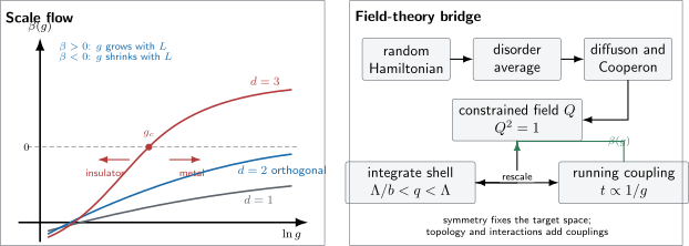
Schematic flow ledger. In the conventional orthogonal class, one and two dimensions flow toward localization, while a three-dimensional curve can cross an unstable fixed point $g_c$. The field-theory route keeps the long-wavelength diffuson and Cooperon sector, packages it in a constrained field $Q$, and integrates momentum shells to obtain the same scale flow. Curve shapes away from controlled asymptotes are qualitative.

Linearized fixed-point flow

It is convenient to write

$$x \equiv \ln g.$$

Near an isolated fixed point $x_c=\ln g_c$,

$$\frac{d(x-x_c)}{d\ln L} = y_g(x-x_c) +O\!\left((x-x_c)^2\right),$$

with

$$y_g = \left. \frac{d\beta}{d\ln g} \right|_{g_c}.$$

The solution is

$$x(L)-x_c \propto L^{y_g}.$$

An unstable transition has $y_g>0$. Matching the scale at which a microscopic detuning becomes order unity gives

$$\nu = \frac{1}{y_g} = \left[ \left. \frac{d\beta}{d\ln g} \right|_{g_c} \right]^{-1}.$$

This relation assumes one relevant direction. If two independent relevant couplings are present, one scalar slope cannot determine the full critical behavior.

One, Two, and Three Dimensions

Dimension and class	Large-scale flow	Interpretation
1D, generic orthogonal	$\beta(g)<0$	Arbitrarily weak uncorrelated disorder produces a finite localization length
2D, orthogonal	$\beta(g)<0$	Weak logarithmic decrease crosses over to exponential localization
2D, unitary without topology	Leading time-reversed correction is removed, but conventional flow is still toward localization	The localization length can be extremely large
2D, symplectic	A metallic regime and an Anderson transition are possible	Spin–orbit coupling changes interference channels and the beta function
2D, quantum Hall or topological classes	Extra topological data are required	Critical extended states and edge structure are not described by a scalar orthogonal beta function
3D, conventional Wigner–Dyson classes	Metal and insulator can be separated by an unstable fixed point	Critical conductance and exponent depend on universality class and convention

One dimension

For a generic one-dimensional random potential, repeated coherent backscattering drives transmission downward at every scale. Even when $g\gg1$ over a short segment, the thermodynamic flow is toward $g=0$. In a quasi-one-dimensional wire with many channels, the localization length can be parametrically larger than the transport mean free path,

$$\xi_{\mathrm{q1D}} \sim N\ell,$$

up to symmetry and boundary factors. The wire can therefore support a long diffusive crossover before exponential localization appears.

“All states localize in one dimension” is not a theorem about every Hamiltonian called one-dimensional. Correlated disorder, special chiral points, quasiperiodicity, protected boundary channels, long-range hopping, and non-Hermitian transport can invalidate the generic assumptions. The Hamiltonian and symmetry class must precede the slogan.

Two dimensions

Two dimensions are marginal at the classical level because $d-2=0$. In the orthogonal class, the negative interference correction makes the beta function negative at large $g$, and the conventional flow has no metallic fixed point. The approach can be logarithmically slow before $L$ reaches the very large localization length.

Breaking time reversal removes the elementary Cooperon contribution, but that fact alone does not guarantee an ordinary two-dimensional metal. In the conventional unitary class, higher-order localization corrections remain. A strong magnetic field can also create Landau levels and a topological term, producing the distinct integer quantum Hall flow with critical extended energies.

Strong spin–orbit coupling places a time-reversal-invariant system in the symplectic class. The weak correction can then be antilocalizing, and a two-dimensional metallic phase separated from an insulator by a critical point is possible. This is why the dimension alone never determines the beta function; dimension and symmetry class form the minimum ledger.

Three dimensions

For $d=3$,

$$\beta(g) \longrightarrow +1 \qquad (g\to\infty),$$

while the localized asymptote is negative. If the flow is continuous, it must cross zero at some $g_c$. The crossing is unstable:

$$\begin{array}{lll} g>g_c &\Longrightarrow& g(L)\ \text{grows},\\[3pt] g<g_c &\Longrightarrow& g(L)\ \text{shrinks}. \end{array}$$

The numerical value of $g_c$ is not universal because it depends on boundaries and conductance normalization. The critical exponent is universal within a specified class. For the standard three-dimensional orthogonal Anderson model, modern finite-size analyses give a benchmark near

$$\nu \simeq 1.57\text{–}1.59,$$

with precise values depending on the model family, observable, corrections-to-scaling ansatz, and quoted uncertainty. That number must not be exported to symplectic, unitary, quantum Hall, chiral, or interacting transitions.

At the fixed point, it is $g(L)$ rather than the bulk conductivity that is scale independent. Rearranging the definition of $g$ gives

$$\sigma_c(L) = \frac{e^2}{h} g_cL^{2-d}.$$

Thus in three dimensions $\sigma_c(L)\propto L^{-1}$ and vanishes in the thermodynamic zero-frequency limit. The metallic side instead reaches a nonzero bulk $\sigma(0)$ after the flow leaves the critical region. Confusing these statements leads to the false expectation that an Anderson critical point should look like an ordinary diffusive metal.

Metal–Insulator Transitions

Relevant and irrelevant variables

Let $u$ measure distance from criticality and choose its sign so that $u>0$ is the metallic side. The diverging correlation or localization length is

$$\xi(u) = \xi_0 \lvert u\rvert^{-\nu}.$$

A realistic finite-size ansatz includes at least one irrelevant variable $v$:

$$g(L,u,v) = \mathcal F \left( uL^{1/\nu}, vL^y \right), \qquad y<0.$$

At $u=0$, the leading term is scale invariant,

$$g(L,0,0)=g_c,$$

but the irrelevant term produces crossing drift at finite $L$. A single clean crossing is suggestive, not a complete exponent analysis.

Near criticality one may expand

$$\ln g(L,u) \simeq \ln g_c +A uL^{1/\nu} +B L^y +\cdots.$$

Fits should vary the minimum size, polynomial order, irrelevant structure, disorder sample count, and covariance treatment. Stability under those choices is part of the result.

Conductivity exponent

On the metallic side in $d>2$, match the critical block at $L\sim\xi$ to ordinary transport at larger scales:

$$g_c \sim \frac{ \sigma(0)\xi^{d-2} }{ e^2/h }.$$

Therefore

$$\sigma(0) \propto \xi^{2-d} \propto u^\mu,$$

with the Wegner scaling relation

$$\mu = (d-2)\nu.$$

This relation belongs to the noninteracting one-parameter framework. Interactions, dangerous irrelevant variables, or additional dynamical scaling can change the relation between a correlation-length exponent and a measured conductivity exponent.

Transfer-matrix finite-size scaling

A common numerical route uses a very long bar with transverse width $M$. From the smallest positive Lyapunov exponent one obtains a quasi-one-dimensional decay length $\lambda_M$. The normalized quantity

$$\Lambda_M \equiv \frac{\lambda_M}{M}$$

obeys a scaling form

$$\Lambda_M = \mathcal G \left( uM^{1/\nu}, vM^y \right).$$

On the localized side, $\Lambda_M$ decreases with $M$; on the metallic side it increases; at criticality it approaches a class-dependent constant. The MacKinnon–Kramer recursive transfer-matrix method made this crossing logic quantitatively practical. The full numerical audit still requires long-bar convergence, uncertainty in Lyapunov exponents, irrelevant fields, energy-window control, and independent fit variants.

A discrete beta-function estimate can be formed from matched sizes:

$$\beta_{\mathrm{eff}} \left( g;L,b \right) = \frac{ \ln g(bL)-\ln g(L) }{ \ln b }.$$

This estimate is meaningful only if both points lie on the same branch of a one-parameter flow. Averaging data from opposite sides of a transition can manufacture a smooth but fictitious beta function.

Broad distributions and critical states

Near localization, conductance and wavefunction intensities are broadly distributed. One-parameter scaling is more faithfully expressed as a flow of the probability distribution,

$$P_L(g) \longrightarrow P_{bL}(g),$$

whose long-distance form is controlled by the same relevant coordinate. At a critical point, the distribution can approach an $L$-independent non-Gaussian shape while wavefunctions remain multifractal. Equality of mean conductance alone does not establish equality of distributions.

For disordered fixed points, the correlation-length exponent is also constrained by disorder-sensitive bounds such as

$$\nu \ge \frac{2}{d}$$

under their stated assumptions. Apparent violations in small systems usually demand a stronger finite-size and correlation audit rather than an immediate claim of new universality.

What an experiment actually scales

An electronic experiment cannot increase coherent length indefinitely. A useful first ledger is

$$L_{\mathrm{eff}} \sim \min \left( L, L_\phi, L_T, L_{\mathrm{escape}} \right),$$

where the relevant thermal length depends on the transport regime. Temperature can tune $L_\phi$, carrier density, interactions, screening, disorder occupation, and phonon scattering simultaneously. A collapse in $T$ and electric field is therefore not automatically the zero-temperature one-parameter flow of a noninteracting Anderson model.

Credible transition evidence combines several diagnostics:

1. a declared Hamiltonian, symmetry class, and tuning parameter;
2. consistent scaling of conductance or normalized localization length over several sizes;
3. explicit irrelevant corrections and crossing-drift tests;
4. localized-side exponential behavior and metallic-side transport behavior;
5. compatible spectral, wavefunction, or boundary-sensitivity diagnostics;
6. robustness to aspect ratio, contacts, disorder realization count, and fit window.

Relation to RG and Quantum Field Theory

The original scaling argument is renormalization-group reasoning expressed directly in an observable. Increasing $L$ removes sensitivity to short-distance details and moves the system along a trajectory in conductance space. Fixed points, relevant perturbations, irrelevant corrections, universality classes, and critical exponents have their usual renormalization-group meaning.

A microscopic field-theory derivation begins with disorder-averaged products of retarded and advanced Green functions. Replica, supersymmetry, or Keldysh methods can perform the disorder average while preserving access to correlation functions. The long-wavelength diffuson and Cooperon modes are encoded in a constrained matrix field

$$Q^2=1.$$

In a common schematic normalization, the nonlinear sigma model has the structure

$$\begin{aligned} S[Q] ={}& \frac{1}{16t} \int d^dr\, \operatorname{Tr} \left( \nabla Q \right)^2 \\ &- \frac{z_\omega\omega}{4} \int d^dr\, \operatorname{Tr} \left( \Lambda Q \right) +S_{\mathrm{top}}[Q] +\cdots, \end{aligned}$$

where

$$t \propto \frac{1}{g}.$$

All prefactors and even the detailed target space depend on convention and symmetry class. The gradient term measures the stiffness of diffusive modes. The frequency term regulates long-time propagation. A topological term, when allowed, can alter the global flow even when the longitudinal conductance is the same.

Integrating a momentum shell and rescaling changes $t$. Since $t\propto1/g$,

$$\frac{d\ln t}{d\ln L} = -\beta(g).$$

Perturbation theory about small $t$ reproduces weak localization and its symmetry-dependent sign. Expansion near $d=2+\epsilon$ organizes the Anderson fixed point when controlled. Nonperturbative configurations and topological terms are essential in several two-dimensional classes.

The sigma model explains both the reach and the limits of a scalar beta function:

• symmetry fixes the manifold of $Q$ and therefore the interference channels;
• interactions add running amplitudes, as in Finkel’stein-type theories;
• topology can add an angle or Wess–Zumino structure;
• frequency and dephasing determine when a static spatial flow is cut off;
• rare events and multifractality require more than a saddle-point conductivity.

This article stops at the quantum-matter consequences of that field theory. Why Many-Body QM Leads to QFT explains the broader emergence of fields and propagators, while Continue on QFT.org provides the publication-aware route to systematic Wilsonian RG and nonlinear-field-theory machinery.

Analysis Workflow

1. Define the conductance. State $G_0$, degeneracies, contact treatment, tensor conversion, boundary conditions, and aspect ratio.
2. Identify microscopic scales. Establish wavelength, mean free path, sample dimensions, and the ballistic-to-diffusive crossover.
3. Fix the symmetry class. Audit time reversal, spin rotation, particle–hole or chiral constraints, magnetic field, and topological sector.
4. Choose a matched ensemble. Hold disorder statistics, energy window, geometry family, and lead protocol fixed across sizes.
5. Select the statistic. Use the mean in a narrow metallic distribution, $\overline{\ln g}$ in a localized distribution, or the full distribution near criticality.
6. Estimate the flow. Compare matched sizes or fit a finite-size scaling function with relevant and irrelevant fields.
7. Test both asymptotes. Look for metallic growth, localized exponential decay, and consistency with perturbative weak localization where applicable.
8. Stress-test the critical fit. Vary size cutoffs, expansion order, irrelevant variables, random samples, covariance model, and optimization starts.
9. Cross-check observables. Compare conductance with localization lengths, level statistics, inverse participation ratios, boundary sensitivity, or wave-packet spreading.
10. State the cutoff. In experiment, report the coherence, thermal, escape, and sample lengths that limit the inferred RG trajectory.

Common Mistakes

• Calling $G$ dimensionless without stating whether it is divided by $e^2/h$ or $2e^2/h$.
• Comparing samples with changing aspect ratio, contacts, channel count, or disorder distribution as though only $L$ changed.
• Treating $\beta_{\mathrm{cl}}=d-2$ as the quantum beta function.
• Extrapolating the perturbative two-dimensional logarithm quantitatively into $g\lesssim1$.
• Saying “all two-dimensional states localize” without specifying the orthogonal, noninteracting, topologically trivial assumptions.
• Identifying every zero of a fitted beta function with a continuous transition without checking stability and extra running variables.
• Reading a critical exponent from one crossing of two sizes.
• Fitting only $\overline g$ when the distribution is broad or log-normal.
• Confusing a spectral band edge with a mobility edge.
• Treating finite-temperature resistance scaling as direct evidence for a zero-temperature noninteracting fixed point.
• Quoting a universal $g_c$; unlike critical exponents, its value depends on conductance and boundary conventions.
• Using a sigma-model action without declaring its symmetry target, normalization, or omitted interaction and topological terms.

Exercises

1. Classical geometric flow

A $d$-dimensional hypercube has size-independent bulk conductivity $\sigma_0$. Derive its dimensionless conductance and classical beta function. Evaluate the result in $d=1,2,3$.

Solution

The conductance of a hypercube scales as

$$G(L) = \sigma_0L^{d-2}.$$

Therefore

$$g(L) = \frac{\sigma_0L^{d-2}}{e^2/h}.$$

Taking a logarithmic derivative gives

$$\beta_{\mathrm{cl}} = \frac{d\ln g}{d\ln L} = d-2.$$

Thus

$$\begin{array}{c|ccc} d&1&2&3\\ \hline \beta_{\mathrm{cl}}&-1&0&+1 \end{array}$$

before quantum corrections are included.

2. Thouless number and conductance

Starting from $E_{\mathrm{Th}}=\hbar D/L^2$, $\Delta_L=[\nu(E_{\mathrm F})L^d]^{-1}$, and $\sigma=e^2\nu(E_{\mathrm F})D$, derive the relation between $g_\sigma$ and $E_{\mathrm{Th}}/\Delta_L$.

Solution

Substitution gives

$$\begin{aligned} g_\sigma &= \frac{\sigma L^{d-2}}{e^2/h}, \\ &= h\nu(E_{\mathrm F})D L^{d-2}. \end{aligned}$$

Meanwhile,

$$\frac{E_{\mathrm{Th}}}{\Delta_L} = \frac{\hbar D}{L^2} \nu(E_{\mathrm F})L^d = \hbar\nu(E_{\mathrm F})D L^{d-2}.$$

Because $h=2\pi\hbar$,

$$g_\sigma = 2\pi \frac{E_{\mathrm{Th}}}{\Delta_L}.$$

The factor $2\pi$ changes if the traversal energy or conductance quantum is normalized differently.

3. Exponentially large two-dimensional crossover

Use

$$\frac{dg}{d\ln L} = -a_2$$

with $a_2=2/\pi$, $g(\ell)=12$, and $g_{\mathrm{cross}}=1$. Estimate $\xi/\ell$.

Solution

Integration gives

$$g(L) = 12-\frac{2}{\pi} \ln \left( \frac{L}{\ell} \right).$$

Set $g(\xi)=1$:

$$\ln \left( \frac{\xi}{\ell} \right) = \frac{11}{2/\pi} = \frac{11\pi}{2} \simeq 17.28.$$

Therefore

$$\frac{\xi}{\ell} \simeq e^{17.28} \simeq 3.2\times10^7.$$

The precise number is not controlled because the weak-coupling equation was extrapolated to $g\sim1$. The robust lesson is the exponential scale separation.

4. Localized asymptote

Suppose

$$g(L) = \left( \frac{L}{\ell} \right)^p \exp \left( -\frac{L}{\xi} \right).$$

Compute $\beta(g)$ as a function of $L$ and show that $\beta\sim\ln g$ for $L\gg\xi$.

Solution

Taking the logarithm,

$$\ln g = p\ln \left( \frac{L}{\ell} \right) -\frac{L}{\xi}.$$

Therefore

$$\beta = \frac{d\ln g}{d\ln L} = p-\frac{L}{\xi}.$$

For $L/\xi\gg1$, the linear term dominates both expressions:

$$\ln g \simeq -\frac{L}{\xi}, \qquad \beta \simeq -\frac{L}{\xi}.$$

Hence $\beta\sim\ln g$ up to subleading logarithmic and constant terms.

5. Fixed-point slope and correlation length

Near an unstable fixed point, let

$$\beta = y_g \left( \ln g-\ln g_c \right), \qquad y_g>0.$$

Show that $\nu=1/y_g$.

Solution

Let

$$\delta x = \ln g-\ln g_c.$$

The flow equation becomes

$$\frac{d\delta x}{d\ln L} = y_g\delta x,$$

so

$$\delta x(L) = \delta x(\ell) \left( \frac{L}{\ell} \right)^{y_g}.$$

If the microscopic detuning is proportional to $u$, the crossover occurs when

$$\lvert u\rvert \xi^{y_g} \sim1.$$

Thus

$$\xi \propto \lvert u\rvert^{-1/y_g}.$$

Comparison with $\xi\propto\lvert u\rvert^{-\nu}$ gives

$$\nu = \frac{1}{y_g}.$$

6. A discrete beta estimate

Matched samples give $g(16a)=3.40$ and $g(32a)=3.15$. Estimate $\beta_{\mathrm{eff}}$ between the two sizes and interpret its sign.

Solution

Here $b=2$, so

$$\begin{aligned} \beta_{\mathrm{eff}} &= \frac{\ln(3.15)-\ln(3.40)}{\ln2}, \\ &\simeq -0.111. \end{aligned}$$

The negative value means the chosen conductance statistic decreases over this scale interval. By itself, one interval does not prove asymptotic localization; larger sizes and a check of one-parameter collapse are required.

7. Classify three two-dimensional flows

For each case, state whether the elementary orthogonal-class conclusion applies:

1. scalar disorder with time reversal and negligible spin–orbit coupling;
2. strong spin–orbit coupling with time reversal preserved;
3. a strong perpendicular field in the integer quantum Hall regime.

Solution

1. This is the conventional orthogonal setting. The large-$g$ correction is localizing, and the thermodynamic flow is toward an insulator.
2. This is a symplectic setting. Weak antilocalization can support a metallic regime and a disorder-driven transition, so the orthogonal conclusion does not apply.
3. Time reversal is broken and Landau-level topology supplies an additional scaling coordinate. Localized states coexist with critical extended energies and chiral edges; a scalar orthogonal beta function is inadequate.

8. Audit a transition claim

A paper reports that resistance curves from four film thicknesses cross at one temperature and collapse when plotted against $(T-T_c)L^{1/\nu}$. List six checks needed before calling the result a noninteracting Anderson transition.

Solution

A sufficient audit should include at least:

1. whether thickness changes only $L$ or also carrier density, disorder, strain, and dimensionality;
2. whether conductance rather than resistance is the correct scaling variable and whether tensor inversion was performed;
3. whether contacts and aspect ratio are matched;
4. whether $L_\phi$, thermal length, and sample dimensions support coherent finite-size scaling;
5. whether interactions, superconducting fluctuations, magnetic scattering, and heating were excluded;
6. whether irrelevant corrections and crossing drift were fitted;
7. whether localized-side exponential transport and metallic-side behavior are independently visible;
8. whether another localization diagnostic supports the same critical point.

The curve collapse is useful evidence, but it does not by itself identify the microscopic universality class.

Connections

• Low-Dimensional Quantum Matter supplies the broader phase-space, fluctuation, and diffusion-return intuition for why dimension changes the infrared problem.
• Anderson Localization develops the microscopic model, localized eigenstates, transfer matrices, dimensional expectations, and direct localization diagnostics.
• Anderson Insulators continues down the localized branch to finite-temperature hopping, Mott and Efros–Shklovskii laws, and parameter-closure tests.
• Mobility Edges applies the critical flow to an energy–disorder boundary and develops multifractal, transfer-matrix, and experimental edge diagnostics.
• Random Matrix Theory in Quantum Matter owns the Poisson, Wigner–Dyson, and critical spectral statistics used to diagnose the flow.
• Weak Localization derives the perturbative large-$g$ correction that fixes the orthogonal two-dimensional beta-function sign.
• Disorder in Quantum Matter defines the disorder ensemble, scattering times, and mean free path at the ultraviolet starting scale.
• Quantum Coherence in Conductors owns $L_\phi$, thermal averaging, escape, and the physical cutoffs of an experimental flow.
• Conductance Quantization derives the Landauer conductance and contact ledger.
• Universal Conductance Fluctuations treats scale-dependent conductance distributions and symmetry crossovers in the coherent diffusive regime.
• Integer Quantum Hall Effect supplies the canonical two-dimensional example in which topology changes localization flow.
• Renormalization Group Preview develops fixed points, relevant and irrelevant directions, universality, and scaling functions in general.
• Finite-Size Scaling in Numerics owns covariance-aware fit design, correction terms, collapse diagnostics, and uncertainty reporting.
• Why Many-Body QM Leads to QFT explains why collective propagators and effective fields emerge from microscopic quantum mechanics.

References

1. D. J. Thouless, “Electrons in Disordered Systems and the Theory of Localization,” Physics Reports 13, 93–142 (1974), doi:10.1016/0370-1573(74)90029-5. Develops boundary sensitivity, transport scales, and early localization criteria.
2. F. J. Wegner, “Electrons in Disordered Systems. Scaling near the Mobility Edge,” Zeitschrift für Physik B 25, 327–337 (1976), doi:10.1007/BF01315248. Establishes critical scaling relations near a mobility edge.
3. E. Abrahams, P. W. Anderson, D. C. Licciardello, and T. V. Ramakrishnan, “Scaling Theory of Localization: Absence of Quantum Diffusion in Two Dimensions,” Physical Review Letters 42, 673–676 (1979), doi:10.1103/PhysRevLett.42.673. Introduces the one-parameter conductance beta function and dimensional flow argument.
4. F. Wegner, “The Mobility Edge Problem: Continuous Symmetry and a Conjecture,” Zeitschrift für Physik B 35, 207–210 (1979), doi:10.1007/BF01319839. Connects the transition to continuous-symmetry field theory.
5. S. Hikami, “Anderson Localization in a Nonlinear-Sigma-Model Representation,” Physical Review B 24, 2671–2679 (1981), doi:10.1103/PhysRevB.24.2671. Develops perturbative localization flow in the nonlinear-sigma-model language.
6. A. MacKinnon and B. Kramer, “One-Parameter Scaling of Localization Length and Conductance in Disordered Systems,” Physical Review Letters 47, 1546–1549 (1981), doi:10.1103/PhysRevLett.47.1546. Establishes recursive transfer-matrix finite-size scaling.
7. P. A. Lee and T. V. Ramakrishnan, “Disordered Electronic Systems,” Reviews of Modern Physics 57, 287–337 (1985), doi:10.1103/RevModPhys.57.287. Reviews interference, scaling, interactions, and experiments.
8. J. T. Chayes, L. Chayes, D. S. Fisher, and T. Spencer, “Finite-Size Scaling and Correlation Lengths for Disordered Systems,” Physical Review Letters 57, 2999–3002 (1986), doi:10.1103/PhysRevLett.57.2999. Proves a disorder-sensitive bound on correlation-length scaling.
9. B. Kramer and A. MacKinnon, “Localization: Theory and Experiment,” Reports on Progress in Physics 56, 1469–1564 (1993), doi:10.1088/0034-4885/56/12/001. Reviews one-parameter scaling, numerical methods, and experimental applications.
10. K. Slevin and T. Ohtsuki, “Corrections to Scaling at the Anderson Transition,” Physical Review Letters 82, 382–385 (1999), doi:10.1103/PhysRevLett.82.382. Demonstrates the importance of irrelevant scaling fields in precision exponent extraction.
11. Y. Asada, K. Slevin, and T. Ohtsuki, “Anderson Transition in Two-Dimensional Systems with Spin-Orbit Coupling,” Physical Review Letters 89, 256601 (2002), doi:10.1103/PhysRevLett.89.256601. Gives a controlled two-dimensional symplectic-class transition.
12. Y. Asada, K. Slevin, and T. Ohtsuki, “Numerical Estimation of the Beta Function in Two-Dimensional Systems with Spin-Orbit Coupling,” Physical Review B 70, 035115 (2004), doi:10.1103/PhysRevB.70.035115. Reconstructs a two-dimensional symplectic beta function numerically.
13. F. Evers and A. D. Mirlin, “Anderson Transitions,” Reviews of Modern Physics 80, 1355–1417 (2008), doi:10.1103/RevModPhys.80.1355. Reviews symmetry classes, field theory, multifractality, and criticality.
14. A. Rodriguez, L. J. Vasquez, K. Slevin, and R. A. Römer, “Multifractal Finite-Size Scaling and Universality at the Anderson Transition,” Physical Review B 84, 134209 (2011), doi:10.1103/PhysRevB.84.134209. Provides precision three-dimensional orthogonal-class benchmarks with covariance-aware scaling.
15. K. Slevin and T. Ohtsuki, “Critical Exponent for the Anderson Transition in the Three-Dimensional Orthogonal Universality Class,” New Journal of Physics 16, 015012 (2014), doi:10.1088/1367-2630/16/1/015012. Refines transfer-matrix estimates and systematic-error controls.

Further Reading

• E. Akkermans and G. Montambaux, Mesoscopic Physics of Electrons and Photons, Cambridge University Press, 2007. A physical route from diffusion modes to weak localization and scaling.
• A. Altland and B. Simons, Condensed Matter Field Theory, 2nd ed., Cambridge University Press, 2010. A systematic replica, supersymmetry, and nonlinear-sigma-model treatment.
• K. B. Efetov, Supersymmetry in Disorder and Chaos, Cambridge University Press, 1997. A technical field-theory account of disorder averaging and localization.