Universal Conductance Fluctuations

Universal conductance fluctuations (UCF) are reproducible, sample-specific variations of the conductance of a phase-coherent disordered conductor as magnetic field, Fermi energy, or impurity configuration is changed. In a fully coherent diffusive metal at zero temperature, their root-mean-square scale is of order $e^2/h$, largely independent of the sample size and elastic disorder strength.

The word fluctuation can be misleading. A magnetoconductance fingerprint, often called a magnetofingerprint, is not ordinarily fluctuating in time: repeated field sweeps reproduce the same irregular pattern while the disorder configuration remains fixed. A different sample, a rearranged impurity, or sometimes a new cooldown produces a different pattern. The randomness belongs to the ensemble of microscopic scattering configurations, while a single frozen sample supplies one reproducible realization.

This page owns the statistics and experimental analysis of sample-specific conductance fingerprints: their interference origin, universal variance, field and energy correlations, symmetry crossover, finite-coherence scaling, and the relation between parameter sweeps and disorder averages. Quantum Coherence in Conductors owns the general dephasing mechanisms and comparison among coherence extractors. Aharonov–Bohm Rings owns flux-periodic winding harmonics. The later disorder and localization chapter will own weak localization and the approach to the Anderson transition.

The Sample-Specific Fingerprint

Let the measured linear-response conductance be $G(X)$, where $X$ may be magnetic field $B$, chemical potential $\mu$, gate voltage $V_g$, or another control parameter. Separate a slowly varying background from the mesoscopic structure:

$$G(X) = G_{\mathrm{smooth}}(X) + \delta G(X).$$

The background may contain Drude magnetoresistance, weak localization, interaction corrections, contact drift, density changes, or a gate-dependent series resistance. UCF refers to the reproducible residual $\delta G$, not to every nonmonotonic feature in the raw trace.

For an ensemble of disorder realizations,

$$\left\langle \delta G \right\rangle_{\mathrm{dis}} = 0,$$

while

$$\operatorname{var}G = \left\langle \delta G^2 \right\rangle_{\mathrm{dis}}$$

remains finite. Experiment usually has one device rather than a fabricated ensemble. A sufficiently broad magnetic-field or gate sweep is therefore used as a surrogate ensemble, subject to conditions discussed below.

Reproducible does not mean immutable

Three measurements should be distinguished:

1. Repeated sweeps with frozen disorder. The same path amplitudes interfere, so the pattern repeats within instrumental and environmental noise.
2. A changed static realization. Charge traps switch, an atom moves, a domain rearranges, or a cooldown changes electrostatics; the new pattern may again be reproducible.
3. Time-dependent noise at fixed controls. The conductance varies during the measurement. UCF can amplify the electrical consequence of moving defects, but the static fingerprint and the defect dynamics are different observables.

The first is the defining experimental signature. The second reveals sensitivity to microscopic configuration. The third belongs to noise spectroscopy and requires a time-correlation or spectral-density analysis.

Conductance convention

For a two-terminal normal conductor in linear response,

$$G = \frac{e^2}{h} g, \qquad g = \operatorname{Tr} \left( t t^\dagger \right) = \sum_n T_n.$$

Here $g$ is dimensionless and every independently counted spin, valley, or other channel is included in the transmission matrix $t$. Some literature instead factors degeneracies out of $g$ or uses $2e^2/h$ as the conductance unit. A quoted UCF coefficient is meaningless unless the conductance unit and degeneracy convention are stated.

The conductance quantum is

$$\frac{e^2}{h} \simeq 38.74\ \mu\mathrm S.$$

UCF is an absolute conductance scale. A good metal can have $\langle G\rangle\gg e^2/h$ while its reproducible mesoscopic variation remains of order $e^2/h$.

Interference Origin

Elastic disorder makes transport diffusive but does not by itself destroy phase coherence. A transmission amplitude from incoming mode $a$ to outgoing mode $b$ may be written schematically as a sum over scattering paths:

$$t_{ba}(B,E) = \sum_\gamma A_\gamma \exp \left[ \frac{i}{\hbar} S_\gamma(E) + i \frac{2\pi B\mathcal A_\gamma}{\Phi_0} \right],$$

where $\mathcal A_\gamma$ is an oriented magnetic area in a convenient gauge-invariant path-pair description and

$$\Phi_0 = \frac{h}{e}$$

is the normal-electron flux quantum.

Squaring the amplitude produces diagonal and interference terms:

$$\lvert t_{ba}\rvert^2 = \sum_\gamma \lvert A_\gamma\rvert^2 + \sum_{\gamma\ne\gamma'} A_\gamma A_{\gamma'}^\ast e^{i\Delta\varphi_{\gamma\gamma'}}.$$

The first sum resembles a classical probability addition. The second depends on relative phases accumulated by many path pairs. For a fixed impurity landscape those phases are fixed, so the interference correction is reproducible.

Changing magnetic field shifts the phase of a pair by

$$\Delta\varphi_{\gamma\gamma'}(B+\Delta B) - \Delta\varphi_{\gamma\gamma'}(B) = 2\pi \frac{\Delta B\,\mathcal A_{\gamma\gamma'}}{\Phi_0}.$$

Changing energy modifies the dynamical phase because paths have different traversal times:

$$\Delta \left( \frac{S_\gamma-S_{\gamma'}}{\hbar} \right) \simeq \frac{\Delta E}{\hbar} \left( t_\gamma-t_{\gamma'} \right).$$

Moving even one sufficiently influential scatterer changes the amplitudes and actions of a large family of paths. These are three ways to sample a correlated interference landscape: vary flux, vary energy, or vary disorder.

Diffusion modes and long-range correlations

Disorder averaging does not simply erase every interference term. In the metallic diffusive regime, correlated retarded and advanced propagators form long-lived diffusion modes. Conductance covariance contains both:

• diffuson contributions, built from paths with the same orientation;
• Cooperon contributions, built from a path and its time reverse.

A schematic correlation kernel has the form

$$C(\Delta E,\Delta B) \propto \operatorname{Re} \sum_{\mathbf q} \frac{1}{ \left[ Dq^2 + \tau_\phi^{-1} + \tau_{\Delta B}^{-1} - i\Delta E/\hbar \right]^2 } + C_{\mathrm C},$$

where $C_{\mathrm C}$ denotes the Cooperon sector and boundary conditions quantize $\mathbf q$. This expression is a structural guide, not a universal fitting formula: current vertices, spin structure, dimensionality, contacts, and geometry determine the prefactors and precise line shape.

The diffusion poles strongly weight long wavelengths. Their infrared enhancement compensates the classical tendency of many regions and channels to self-average. That cancellation is the central reason an order-unity variance of $g$ survives in a coherent diffusive sample.

What Universality Means

The simplest UCF regime satisfies

$$\ell \ll L \ll \xi, \qquad k_{\mathrm F}\ell \gg 1, \qquad \langle g\rangle \gg 1,$$

where $\ell$ is the elastic mean free path, $L$ is the relevant sample length, and $\xi$ is the localization length. The sample must also be coherent and not thermally averaged across many independent spectral intervals:

$$L \lesssim L_\phi, \qquad L \lesssim L_T,$$

with

$$L_T = \sqrt{ \frac{\hbar D}{k_{\mathrm B}T} }.$$

In this window,

$$\operatorname{rms}\delta G = \sqrt{ \left\langle \delta G^2 \right\rangle } \sim \frac{e^2}{h}.$$

The elastic mean free path and average Drude conductance may vary greatly while the fluctuation scale remains quantum mechanical.

A precise quasi-one-dimensional benchmark

For a standard spin-resolved channel convention, a long coherent quasi-one-dimensional diffusive wire with ideal leads has

$$\operatorname{var}g = \frac{2}{15\beta},$$

where $\beta=1$ for the orthogonal symmetry class and $\beta=2$ for the unitary class. Thus,

$$\operatorname{rms}\delta G = \frac{e^2}{h} \sqrt{ \frac{2}{15\beta} }.$$

This benchmark is powerful precisely because its assumptions are narrow. Geometry, finite aspect ratio, contact resistance, spin and valley degeneracy, spin–orbit coupling, intervalley scattering, nonideal leads, and measurement configuration change the coefficient. A ballistic chaotic cavity has a different universal variance from a diffusive wire.

Magnetic symmetry crossover

At zero magnetic field and without magnetic disorder, both diffuson and Cooperon sectors contribute. A sufficiently large mean field breaks time-reversal symmetry and suppresses the Cooperon. In the simplest orthogonal-to-unitary crossover,

$$\operatorname{var}G_{\mathrm{unitary}} \simeq \frac{1}{2} \operatorname{var}G_{\mathrm{orthogonal}},$$

so the rms amplitude falls by

$$\operatorname{rms}\delta G_{\mathrm{unitary}} \simeq \frac{1}{\sqrt 2} \operatorname{rms}\delta G_{\mathrm{orthogonal}}.$$

Spin degeneracy, Zeeman splitting, spin–orbit coupling, valleys, and partially gapped diffusion modes can add further crossovers. A measured factor need not equal the textbook value unless those modes are counted explicitly.

What is not universal

The following are not universal:

• the detailed positions of peaks and valleys;
• the peak-to-peak span of a finite sweep;
• the smooth background under the fingerprint;
• the field or gate correlation scale;
• the coefficient for an arbitrary geometry and contact layout;
• the fluctuation distribution near localization or a conductance threshold;
• an apparent amplitude extracted from too few independent features.

Universality concerns a variance in a stated ensemble and symmetry class. It does not turn one irregular trace into a parameter-free prediction.

Finite Coherence and Thermal Averaging

Real devices are often longer than $L_\phi$. Coherence is then limited to subregions, and classical composition of their conductances reduces the terminal fluctuation amplitude.

For a roughly hypercubic $d$-dimensional diffusive sample of linear size $L$, in the regime

$$\ell \ll L_\phi \ll L, \qquad L_\phi \lesssim L_T,$$

the scaling form is

$$\operatorname{rms}\delta G \sim C_d \frac{e^2}{h} \left( \frac{L_\phi}{L} \right)^{(4-d)/2}.$$

$C_d$ is an order-unity geometry and symmetry factor. The exponent is $3/2$ in quasi-one dimension, $1$ in two dimensions, and $1/2$ in three dimensions. Rectangular devices require the actual series and parallel network of coherence volumes rather than blindly inserting one $L$.

For a quasi-one-dimensional wire of length $L$ and transverse dimensions shorter than $L_\phi$ and $L_T$,

$$\operatorname{rms}\delta G \sim C_1 \frac{e^2}{h} \left( \frac{L_\phi}{L} \right)^{3/2}, \qquad L_\phi \lesssim L_T.$$

When thermal averaging is stronger,

$$\operatorname{rms}\delta G \sim C_T \frac{e^2}{h} \frac{L_T}{L} \left( \frac{L_\phi}{L} \right)^{1/2}, \qquad L_T \ll L_\phi \ll L.$$

These are scaling laws, not drop-in calibration equations. Published prefactors depend on how $L_\phi$, $L_T$, conductance, and the experimental variance are defined.

Thermal averaging is not dephasing

The finite-temperature linear conductance is

$$G(T) = \int dE\, \left( -\frac{\partial f}{\partial E} \right) G_0(E).$$

This averages a coherent zero-temperature fingerprint $G_0(E)$ over an energy window of order $k_{\mathrm B}T$. Separately, temperature-dependent interactions or phonons shorten $\tau_\phi$ and hence

$$L_\phi = \sqrt{ D\tau_\phi }.$$

Both effects reduce the observed variance, but only the second destroys phase memory. A fit that assigns the entire temperature dependence to $L_\phi(T)$ can systematically underestimate coherence.

Magnetic-Field Correlations

Define the field autocovariance after background subtraction:

$$C_B(\Delta B) = \left\langle \delta G(B) \delta G(B+\Delta B) \right\rangle_B.$$

Then

$$C_B(0) = \operatorname{var}_B G,$$

and a common correlation-field convention is

$$C_B(B_c) = \frac{1}{2} C_B(0).$$

Other conventions use a $1/e$ width, the first zero, or an integral correlation scale. Numerical prefactors cannot be compared until the convention is matched.

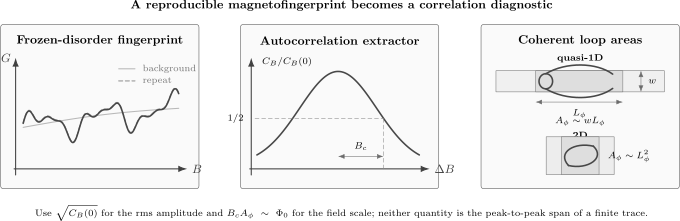
A frozen disorder configuration produces a repeatable aperiodic fingerprint. Its rms amplitude is $\sqrt{C_B(0)}$, while the correlation width $B_c$ estimates the coherent loop area through $B_cA_\phi\sim\Phi_0$. In a narrow wire $A_\phi\sim wL_\phi$; in a two-dimensional sheet $A_\phi\sim L_\phi^2$, up to geometry and width-convention factors.

Flux through a coherence area

Field decorrelates the path sum when it threads roughly one flux quantum through a typical coherent loop:

$$B_cA_\phi \sim \Phi_0.$$

For a perpendicular field in a quasi-one-dimensional wire of width $w$,

$$A_\phi \sim wL_\phi, \qquad B_c \sim \alpha_{1\mathrm D} \frac{\Phi_0}{wL_\phi}.$$

For a two-dimensional coherent patch,

$$A_\phi \sim L_\phi^2, \qquad B_c \sim \alpha_{2\mathrm D} \frac{\Phi_0}{L_\phi^2}.$$

The coefficients $\alpha_{1\mathrm D}$ and $\alpha_{2\mathrm D}$ depend on boundary scattering, field orientation, dimensional crossover, and the definition of $B_c$. The electronic width can also differ from the lithographic width.

Example. A narrow wire has $w=80\ \mathrm{nm}$ and a half-height correlation field $B_c=0.30\ \mathrm T$. Taking $\alpha_{1\mathrm D}=1$ for an order-of-magnitude estimate gives

$$L_\phi \sim \frac{\Phi_0}{wB_c} \simeq 1.72\times10^{-7}\ \mathrm m = 172\ \mathrm{nm}.$$

This estimate is not yet a precision measurement. It must be corrected with the appropriate geometry factor and compared with weak-localization or ring-based coherence extraction.

Mean field and field difference do different jobs

Two field scales enter:

1. The mean field $B_0$ changes the symmetry class by suppressing time-reversed interference.
2. The difference field $\Delta B$ decorrelates two fingerprints being compared.

In diagrammatic language, the diffuson depends mainly on the field difference, while the Cooperon depends on a field sum. Treating these as one scale obscures the factor-of-two variance crossover.

For a two-terminal conductor in linear response,

$$G(B) = G(-B)$$

by Onsager–Casimir reciprocity. The negative- and positive-field halves are therefore mirror related, not independent disorder samples. A field window from $-B_{\max}$ to $B_{\max}$ does not automatically provide twice as many independent UCF features as $0$ to $B_{\max}$.

Energy, Gate, and Bias Correlations

An energy autocovariance can be defined by

$$C_E(\Delta E) = \left\langle \delta G(E) \delta G(E+\Delta E) \right\rangle_E.$$

The natural decorrelation scale is the Thouless energy of the largest coherently explored region:

$$E_c \sim \frac{\hbar D}{L_{\mathrm{eff}}^2}, \qquad L_{\mathrm{eff}} \sim \min \left( L, L_\phi \right),$$

with geometry-dependent factors. When transverse dimensions or dwell time set the slowest diffusion mode, they must be included explicitly.

Example. For $D=0.020\ \mathrm{m^2\,s^{-1}}$ and $L_{\mathrm{eff}}=0.50\ \mu\mathrm m$,

$$E_c \sim \frac{ \hbar(0.020\ \mathrm{m^2\,s^{-1}}) }{ (0.50\ \mu\mathrm m)^2 } \simeq 52.7\ \mu\mathrm{eV}.$$

The corresponding temperature is

$$\frac{E_c}{k_{\mathrm B}} \simeq 0.61\ \mathrm K.$$

Thermal averaging becomes important well before a bath-temperature sweep can be interpreted as pure dephasing if $k_{\mathrm B}T\gtrsim E_c$.

Gate voltage is not energy until calibrated

If a gate shifts the relevant electrochemical potential by

$$\Delta E = \alpha_g e\,\Delta V_g,$$

then a gate correlation voltage $V_c$ can estimate

$$E_c \sim \alpha_g eV_c.$$

But a gate may also change:

• carrier density and diffusion constant;
• transverse mode occupation;
• contact transmission;
• screening of the disorder potential;
• trap occupation and the disorder realization itself.

A lever arm from Coulomb diamonds, compressibility, capacitance, or finite-bias spectroscopy is preferable to assuming $\alpha_g=1$.

Finite source–drain bias samples an energy interval of order $e\lvert V\rvert$ and may also heat the electrons or drive a nonequilibrium distribution. Nonlinear conductance fluctuations are therefore not obtained by merely replacing $k_{\mathrm B}T$ with $eV$.

Disorder Averaging and Ergodicity

Theory commonly computes

$$C_{\mathrm{dis}}(\Delta X) = \left\langle \delta G(X;U) \delta G(X+\Delta X;U) \right\rangle_U,$$

where $U(\mathbf r)$ labels the random potential. Experiment more often computes an average over $X$ in one sample. Equating the two is an ergodic hypothesis: changing field or energy is assumed to explore the same fluctuation statistics as changing disorder.

This can work well in the diffusive metallic regime when:

• the sweep spans many correlation fields or energies;
• the smooth classical response is removed without erasing UCF;
• the device remains in one transport regime;
• contacts and disorder remain stationary;
• symmetry changes across the window are treated separately.

It can fail when a gate moves charge traps, a wide field sweep changes orbital transport or spin polarization, a transition is crossed, or the available range contains only a few independent features.

Several distinct averages

Average	What changes	What it estimates	Main caveat
fabricated ensemble	microscopic disorder between devices	disorder statistics directly	geometry and contacts also vary
cooldown ensemble	frozen electrostatic configuration	approximate disorder ensemble	density and contact state may change
field average	orbital phase	correlation and variance in one device	mean field changes symmetry and background
gate average	energy and often density	energy correlation if calibrated	disorder and modes may also change
thermal average	occupied energy window	finite-temperature conductance	not a disorder realization
time average	dynamic environment	noise or drift statistics	erases the static fingerprint if defects move

An average is not made trustworthy by having many data points. The number of statistically useful samples is set by the correlation scale.

If a one-sided field interval has usable width $W_B$, a rough count is

$$N_{\mathrm{eff}} \sim \frac{W_B}{B_c}.$$

Oversampling the trace more finely does not increase $N_{\mathrm{eff}}$. Background fitting and long correlation tails usually reduce it further.

A Practical Analysis Workflow

1. Preserve the raw measurement

Record sweep direction, excitation current or voltage, lock-in frequency, gate history, temperature, and field ramp rate. Repeat the sweep before filtering. A fingerprint that does not repeat is not ready for a UCF variance analysis.

2. Convert resistance carefully

For a two-terminal measurement,

$$G = \frac{1}{R}$$

only after identifying series resistance and the relevant differential quantity. For small resistance changes around $R_0$,

$$\delta G \simeq -\frac{\delta R}{R_0^2},$$

but this linearization fails for large variations. Four-terminal resistance is not automatically the inverse of a two-terminal Landauer conductance.

3. Define the background transparently

Choose a smoothing scale much broader than the expected UCF correlation field. Repeat the analysis with several defensible polynomial orders, splines, or filter widths. Report how $\operatorname{rms}\delta G$ and $B_c$ change.

Subtracting a high-temperature trace can be useful only if the classical background is stable. Temperature also changes density, weak localization, interactions, and contacts, so the subtraction can introduce structure.

4. Compute covariance without circular normalization

Evaluate $C_B(\Delta B)$ from the residual over a stationary window. Use

$$\operatorname{rms}\delta G = \sqrt{C_B(0)}$$

before normalizing the curve. Then state the width convention used for $B_c$.

5. Separate symmetry sectors

Do not estimate one variance across a field window that straddles the time-reversal crossover unless the crossover is modeled. Compare low- and high-mean-field windows with similar widths and backgrounds when testing the predicted variance reduction.

6. Propagate geometric and statistical uncertainty

Uncertainty in $w$, field angle, conducting thickness, lever arm, $D$, and background choice enters $L_\phi$ or $E_c$. A credible result reports these alongside finite-window uncertainty from the limited number of independent features.

7. Cross-check another coherence observable

Compare the inferred $L_\phi(T)$ with weak localization, Aharonov–Bohm harmonics, or another geometry. Agreement in trend and scale is stronger than forcing identical prefactors onto observables with different path weighting.

Distinguishing Nearby Phenomena

Phenomenon	Pattern	Parameter periodicity	Averaging behavior	Primary diagnostic
universal conductance fluctuations	reproducible and aperiodic	correlated in $B$ and $E$, not periodic	sample-specific mean is removed; variance survives	$C_B$, $C_E$, rms scale
Aharonov–Bohm oscillations	reproducible harmonics	periodic in flux $BA_{\mathrm{eff}}$	winding peaks can survive suitable averaging	$h/e$ and $h/2e$ Fourier components
weak localization	smooth low-field cusp	no oscillation period	survives disorder averaging	centered magnetoconductance line shape
Shubnikov–de Haas oscillations	oscillatory at higher field	periodic in $1/B$	tied to Landau quantization	frequency versus Fermi-surface area
telegraph or $1/f$ noise	changes with time at fixed controls	frequency-domain statistics	time average is essential	time trace and noise spectrum
classical magnetoresistance	smooth material response	generally nonperiodic	reproducible across disorder realizations	mobility and tensor transport model

An irregular trace is not automatically UCF. Reproducibility, covariance, temperature evolution, geometry scaling, and exclusion of periodic or time-dependent alternatives form the evidence.

Common Mistakes

• Calling a reproducible field trace measurement noise.
• Quoting the largest peak-to-peak excursion as the UCF amplitude instead of using $\sqrt{C_B(0)}$.
• Saying the rms value is always exactly $e^2/h$ without specifying symmetry, geometry, degeneracy, and contacts.
• Using both halves of an even two-terminal trace as independent samples.
• Extracting $L_\phi$ from $B_c$ without stating the width convention or geometry factor.
• Treating thermal averaging and microscopic dephasing as the same process.
• Assuming a gate sweep changes only Fermi energy.
• Detrending with a scale comparable to $B_c$, thereby removing the signal being measured.
• Interpreting every aperiodic feature in a topological material as evidence for topological boundary transport.
• Applying diffusive UCF formulas in a ballistic cavity, hopping conductor, Coulomb-blockaded device, or strongly localized regime.

Exercises

1. Magnetic phase of a path pair

Two interfering diffusive paths enclose oriented area $\mathcal A=0.060\ \mu\mathrm m^2$. Estimate the field change that shifts their relative phase by $2\pi$.

Solution

The phase change is

$$\Delta\varphi = 2\pi \frac{\Delta B\,\mathcal A}{\Phi_0}.$$

Setting $\Delta\varphi=2\pi$ gives

$$\Delta B = \frac{\Phi_0}{\mathcal A} = \frac{ 4.136\times10^{-15}\ \mathrm{Wb} }{ 0.060\times10^{-12}\ \mathrm{m^2} } \simeq 6.89\times10^{-2}\ \mathrm T.$$

Thus $\Delta B\simeq69\ \mathrm{mT}$. A real UCF correlation field averages over a distribution of path-pair areas, so this is an area-scale estimate rather than a predicted oscillation period.

2. Coherence length from a field correlation

A quasi-one-dimensional wire has electronic width $w=120\ \mathrm{nm}$ and half-height correlation field $B_c=0.18\ \mathrm T$. Estimate $L_\phi$ using $B_cwL_\phi=\Phi_0$. State the main systematic caveat.

Solution

Solving gives

$$L_\phi = \frac{\Phi_0}{wB_c} = \frac{ 4.136\times10^{-15}\ \mathrm{Wb} }{ (120\times10^{-9}\ \mathrm m)(0.18\ \mathrm T) } \simeq 1.91\times10^{-7}\ \mathrm m.$$

Therefore

$$L_\phi \simeq 191\ \mathrm{nm}.$$

The dominant systematic caveat is the geometry factor: the half-height convention, boundary scattering, field angle, and difference between electronic and lithographic width change the coefficient multiplying $\Phi_0/(wB_c)$.

3. Finite-coherence amplitude

A quasi-one-dimensional wire has $L=2.0\ \mu\mathrm m$, $L_\phi=0.50\ \mu\mathrm m$, and $L_T\gtrsim L_\phi$. Taking $C_1=1$, estimate $\operatorname{rms}\delta G$.

Solution

Use

$$\operatorname{rms}\delta G \sim \frac{e^2}{h} \left( \frac{L_\phi}{L} \right)^{3/2}.$$

Since $L_\phi/L=0.25$,

$$\left( 0.25 \right)^{3/2} = 0.125.$$

Hence

$$\operatorname{rms}\delta G \sim 0.125 \frac{e^2}{h} \simeq 4.84\ \mu\mathrm S.$$

This is a scaling estimate. A quantitative comparison needs the symmetry, degeneracy, contact, and geometry prefactor.

4. Breaking time-reversal symmetry

The low-field rms fluctuation is $0.70\,e^2/h$. If breaking time-reversal symmetry halves the variance and no other diffusion mode changes, what high-field rms value is expected?

Solution

Variance is the square of the rms amplitude. Therefore halving the variance reduces the rms by $1/\sqrt2$:

$$\operatorname{rms}\delta G_{\mathrm{high}} = \frac{ 0.70 }{ \sqrt2 } \frac{e^2}{h} \simeq 0.495 \frac{e^2}{h}.$$

The rms does not fall by a factor of two. Observing another ratio may signal spin, valley, Zeeman, spin–orbit, or incomplete symmetry crossover effects.

5. Energy correlation scale

For a coherent diffusive region with $D=0.015\ \mathrm{m^2\,s^{-1}}$ and $L_{\mathrm{eff}}=300\ \mathrm{nm}$, estimate $E_c=\hbar D/L_{\mathrm{eff}}^2$ in $\mu\mathrm{eV}$ and $E_c/k_{\mathrm B}$ in kelvin.

Solution

The Thouless scale is

$$E_c = \frac{ (1.055\times10^{-34}\ \mathrm{J\,s}) (0.015\ \mathrm{m^2\,s^{-1}}) }{ (300\times10^{-9}\ \mathrm m)^2 } \simeq 1.76\times10^{-23}\ \mathrm J.$$

Dividing by the elementary charge gives

$$E_c \simeq 1.10\times10^{-4}\ \mathrm{eV} = 110\ \mu\mathrm{eV}.$$

Therefore

$$\frac{E_c}{k_{\mathrm B}} \simeq 1.27\ \mathrm K.$$

Geometry-dependent eigenvalue factors can shift both numbers.

6. Counting independent field features

A two-terminal trace is measured from $-1.2\ \mathrm T$ to $1.2\ \mathrm T$, and $B_c=0.08\ \mathrm T$. The trace is even in $B$. Estimate the number of independent field intervals before accounting for long correlation tails.

Solution

Because

$$G(B) = G(-B),$$

the two halves are mirrored and should not be counted independently. The independent one-sided width is approximately $1.2\ \mathrm T$, so

$$N_{\mathrm{eff}} \sim \frac{ 1.2\ \mathrm T }{ 0.08\ \mathrm T } = 15.$$

Counting the full $2.4\ \mathrm T$ width would double-count reciprocal data. Background fitting and correlations beyond $B_c$ can reduce the effective count below $15$.

7. Thermal averaging or dephasing?

The UCF rms amplitude decreases with temperature while $B_c$ remains nearly constant. Give one plausible interpretation and one check.

Solution

If $B_c$ is controlled by $L_\phi$ and remains constant, the decreasing amplitude may be dominated by thermal energy averaging rather than a shortening of $L_\phi$. This is plausible when $k_{\mathrm B}T$ exceeds the energy correlation scale while the microscopic dephasing rate changes weakly.

A check is to measure the energy or gate correlation scale and compare $k_{\mathrm B}T$ with $E_c$. One can also compare $L_\phi(T)$ extracted from weak localization. Stable $B_c$ and weak-localization width together with falling UCF variance would support the thermal-averaging interpretation.

8. Classify three traces

Trace A is reproducible and periodic in $B$. Trace B is reproducible, aperiodic, and has a finite field autocorrelation width. Trace C changes between repeated sweeps at the same controls and has a broad low-frequency spectrum. Classify the most likely primary phenomenon in each case.

Solution

• Trace A: a flux-periodic interference effect such as Aharonov–Bohm oscillations, subject to checking the area and harmonic content.
• Trace B: universal conductance fluctuations, subject to verifying the order-$e^2/h$ scale, temperature evolution, and diffusive regime.
• Trace C: time-dependent conductance noise or drift, possibly produced by fluctuating defects whose electrical sensitivity is enhanced by mesoscopic interference.

The categories can coexist. A ring may show an Aharonov–Bohm peak on top of UCF, and slowly moving scatterers can make the UCF fingerprint evolve in time.

Connections

• What Is Mesoscopic Physics? supplies the wavelength, mean-free-path, coherence, thermal, Thouless, dwell, and contact hierarchy.
• Quantum Coherence in Conductors owns microscopic dephasing, $L_\phi$, $L_T$, weak-localization comparison, and low-temperature saturation controls.
• Weak Localization derives the ensemble-averaged Cooperon correction and field scale that complement the sample-specific covariance treated here.
• Disorder in Quantum Matter supplies the quenched-ensemble and random-potential statistics whose sample fingerprints are compared in fluctuation measurements.
• Anderson Localization owns the strong-localization regime where conductance distributions broaden and $\overline{\ln g}$, rather than order-$e^2/h$ variance, becomes the central scaling observable.
• Scaling Theory of Localization organizes the size evolution of conductance statistics and distinguishes a scalar running coordinate from the full critical distribution.
• Random Matrix Theory in Quantum Matter develops the invariant Gaussian and circular ensembles underlying zero-dimensional spectral and scattering universality.
• Aharonov–Bohm Rings separates aperiodic UCF from flux-periodic $h/e$ and $h/2e$ winding harmonics.
• Conductance Quantization derives the Landauer formula, transmission eigenvalues, channel counting, contact resistance, and shot noise.
• Quantum Wires develops the transverse subbands and effective one-dimensional geometry used in the quasi-one-dimensional scaling laws.
• Two-Dimensional Electron Gases supplies density, mobility, diffusion, Hall, lifetime, and gate-calibration context for semiconductor UCF experiments.
• Graphene and Dirac Materials explains valley, intervalley, spin, and Dirac-band structure that can modify the diffusion-mode count.
• One-over-f Noise owns stationary time-correlation functions, power spectra, fluctuator ensembles, and the distinction between static fingerprints and temporal noise.
• Mesoscopic Transport develops reservoir dynamics, counting statistics, and detector backaction beyond elastic linear response.
• Conventions for Quantum Matter fixes charge, current, response, and Fourier conventions.

Further Reading

• E. Akkermans and G. Montambaux, Mesoscopic Physics of Electrons and Photons, Cambridge University Press, 2007, especially Chapter 11.
• Y. Imry, Introduction to Mesoscopic Physics, 2nd ed., Oxford University Press, 2002.
• S. Datta, Electronic Transport in Mesoscopic Systems, Cambridge University Press, 1995.
• C. W. J. Beenakker, “Random-Matrix Theory of Quantum Transport,” Reviews of Modern Physics 69, 731–808 (1997), doi:10.1103/RevModPhys.69.731.

References

1. C. P. Umbach, S. Washburn, R. B. Laibowitz, and R. A. Webb, “Magnetoresistance of Small, Quasi-One-Dimensional, Normal-Metal Rings and Lines,” Physical Review B 30, 4048–4051 (1984), doi:10.1103/PhysRevB.30.4048.
2. A. D. Stone, “Magnetoresistance Fluctuations in Mesoscopic Wires and Rings,” Physical Review Letters 54, 2692–2695 (1985), doi:10.1103/PhysRevLett.54.2692.
3. B. L. Altshuler, “Fluctuations in the Extrinsic Conductivity of Disordered Conductors,” JETP Letters 41, 648–651 (1985).
4. P. A. Lee and A. D. Stone, “Universal Conductance Fluctuations in Metals,” Physical Review Letters 55, 1622–1625 (1985), doi:10.1103/PhysRevLett.55.1622.
5. B. L. Altshuler and D. E. Khmelnitskii, “Fluctuation Properties of Small Conductors,” JETP Letters 42, 359–362 (1985).
6. J. C. Licini, D. J. Bishop, M. A. Kastner, and J. Melngailis, “Aperiodic Magnetoresistance Oscillations in Narrow Inversion Layers in Si,” Physical Review Letters 55, 2987–2990 (1985), doi:10.1103/PhysRevLett.55.2987.
7. W. J. Skocpol, P. M. Mankiewich, R. E. Howard, L. D. Jackel, D. M. Tennant, and A. D. Stone, “Universal Conductance Fluctuations in Silicon Inversion-Layer Nanostructures,” Physical Review Letters 56, 2865–2868 (1986), doi:10.1103/PhysRevLett.56.2865.
8. S. Feng, P. A. Lee, and A. D. Stone, “Sensitivity of the Conductance of a Disordered Metal to the Motion of a Single Atom: Implications for $1/f$ Noise,” Physical Review Letters 56, 1960–1963 (1986), doi:10.1103/PhysRevLett.56.1960.
9. P. A. Lee, A. D. Stone, and H. Fukuyama, “Universal Conductance Fluctuations in Metals: Effects of Finite Temperature, Interactions, and Magnetic Field,” Physical Review B 35, 1039–1070 (1987), doi:10.1103/PhysRevB.35.1039.
10. T. J. Thornton, M. Pepper, H. Ahmed, G. J. Davies, and D. Andrews, “Universal Conductance Fluctuations and Electron Coherence Lengths in a Narrow Two-Dimensional Electron Gas,” Physical Review B 36, 4514–4517 (1987), doi:10.1103/PhysRevB.36.4514.
11. P. A. Mello, P. Pereyra, and N. Kumar, “Macroscopic Approach to Multichannel Disordered Conductors,” Annals of Physics 181, 290–317 (1988), doi:10.1016/0003-4916(88)90169-8.
12. N. Argaman, “Semiclassical Analysis of the Quantum Interference Corrections to the Conductance of Mesoscopic Systems,” Physical Review B 53, 7035–7064 (1996), doi:10.1103/PhysRevB.53.7035.