Anderson Localization

Anderson localization is the suppression of wave transport by coherent multiple scattering from static disorder. It can occur without a band gap, a classical barrier, or particle–particle interactions. The disorder randomizes the phases accumulated along different paths, yet the resulting interference is not featureless: repeated scattering can organize amplitudes into spatially localized eigenstates and prevent an initially compact wave packet from diffusing indefinitely.

The central claim is stronger than “the mean free path is short.” Elastic scattering first destroys momentum memory and produces diffusion. Localization concerns what phase-coherent interference does to that diffusion on still longer scales.

This page owns Anderson localization as a single-particle quantum-matter phenomenon: the benchmark lattice model, exponential localization, transfer matrices, dimensional dependence, diagnostics, and evidence standards. Disorder in Quantum Matter owns disorder ensembles and scattering lifetimes. Quantum Coherence in Conductors owns dephasing and the diffusive coherence hierarchy. Scaling Theory of Localization owns beta-function flow, Anderson Insulators owns localized-side hopping transport, and Mobility Edges owns the energy–disorder boundary and its critical analysis.

Three Operational Meanings

Localization is best established by several compatible statements rather than by one visual impression.

Eigenstate localization

For a normalized one-particle eigenstate centered near $\mathbf r_\alpha$, an exponentially localized envelope obeys

$$\lvert\psi_\alpha(\mathbf r)\rvert \lesssim C_\alpha \exp\!\left( -\frac{\lvert\mathbf r-\mathbf r_\alpha\rvert}{\xi_\alpha} \right)$$

outside a microscopic core. The localization length $\xi_\alpha$ is energy-, disorder-, and symmetry-dependent. Oscillations and rare resonant peaks can sit beneath the envelope, so a straight-line fit to a short semilog tail is not by itself decisive.

Dynamical localization

Launch a state $\lvert\mathbf r_0\rangle$ and define its second spatial moment,

$$m_2(t) = \sum_{\mathbf r} \lvert\mathbf r-\mathbf r_0\rvert^2 \left| \langle\mathbf r| e^{-i\hat Ht/\hbar} |\mathbf r_0\rangle \right|^2.$$

Ordinary diffusion gives

$$\overline{m_2(t)} \simeq 2dDt$$

after microscopic transients. In a dynamically localized regime, the packet may spread initially, but its long-time spatial moments remain bounded under appropriate disorder and energy averaging:

$$\limsup_{t\to\infty} \overline{m_2(t)} < \infty.$$

Localization therefore means absence of unbounded diffusion, not absence of all microscopic motion.

Transport localization

Attach ideal leads and form the dimensionless two-terminal conductance

$$g = \frac{G}{e^2/h} = \operatorname{Tr} \left( t^\dagger t \right),$$

where $t$ is the transmission matrix and spin or valley factors must be declared separately. In a long localized sample, the typical conductance

$$g_{\mathrm{typ}} \equiv \exp\!\left( \overline{\ln g} \right)$$

falls exponentially with length. One common quasi-one-dimensional convention is

$$\overline{\ln g} \sim -\frac{2L}{\xi_{\mathrm{tr}}}.$$

Some authors absorb the factor of $2$ into the definition of the transport localization length. A reported $\xi$ is incomplete unless its estimator is stated.

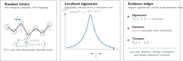
Three views of Anderson localization. Random on-site energies compete with hopping $t$; a localized eigenstate has an exponential probability envelope set by $\xi$; and a credible diagnosis combines eigenstate, dynamical, and transport scaling rather than relying on one insulating-looking trace.

Interference and the Absence of Diffusion

A propagator through a disordered region can be organized schematically as a sum over multiple-scattering paths $\mathcal P$,

$$K(\mathbf r_f,\mathbf r_i;t) = \sum_{\mathcal P} A_{\mathcal P} e^{i\phi_{\mathcal P}}.$$

Its probability contains diagonal and interference terms:

$$\lvert K\rvert^2 = \sum_{\mathcal P} \lvert A_{\mathcal P}\rvert^2 + \sum_{\mathcal P\ne\mathcal P'} A_{\mathcal P}A_{\mathcal P'}^\ast e^{i(\phi_{\mathcal P}-\phi_{\mathcal P'})}.$$

A classical random walk retains only the first sum. A disorder average suppresses many cross terms, but not all of them. Time-reversed loops, repeated returns, and families of paths constrained by symmetry retain correlated phases. Their cumulative effect changes transport at scales larger than the elastic mean free path.

The hierarchy is

$$\text{ballistic} \;\longrightarrow\; \text{diffusive} \;\longrightarrow\; \text{localized},$$

with the last crossover possible only while phase information survives. If the phase-coherence length $L_\phi$ is shorter than the localization length, dephasing truncates the interference buildup and the sample can display only a precursor. Magnetic flux, spin–orbit coupling, and internal symmetries also change which path pairs interfere, so dimensionality alone never specifies the localization class.

Weak localization is the perturbative correction produced by a restricted set of coherent return paths while $g\gg1$. Anderson localization is the nonperturbative regime in which transmission itself becomes exponentially small. The two are connected, but fitting a small magnetoconductance cusp does not establish strong localization.

The Anderson Model

The standard tight-binding benchmark is

$$\hat H = \sum_i \epsilon_i \lvert i\rangle\langle i\rvert - \sum_{\langle i,j\rangle} \left( t_{ij}\lvert i\rangle\langle j\rvert + t_{ij}^\ast\lvert j\rangle\langle i\rvert \right).$$

The simplest diagonal-disorder Anderson model uses a regular lattice, nearest-neighbor hopping $t_{ij}=t$, and independent site energies drawn from

$$P(\epsilon) = \begin{cases} 1/W, & -W/2\le\epsilon\le W/2,\\ 0, & \text{otherwise}. \end{cases}$$

Then

$$\overline{\epsilon_i}=0, \qquad \overline{\epsilon_i\epsilon_j} = \frac{W^2}{12}\delta_{ij}.$$

Only dimensionless combinations such as $W/t$, $E/t$, and $L/a$ can be compared across calculations. Replacing the box distribution by a Gaussian, correlating nearby $\epsilon_i$, randomizing the hoppings, adding magnetic phases, or adding spin–orbit matrices defines a different model. Universal critical behavior may survive some changes, but mobility edges and microscopic localization lengths generally do not.

For a clean hypercubic lattice,

$$E(\mathbf k) = -2t \sum_{\mu=1}^{d} \cos(k_\mu a).$$

The eigenstates are extended Bloch waves. In the opposite atomic limit $t=0$, each nondegenerate site orbital is an exact localized eigenstate. Anderson localization describes the interference-controlled connection between these limits; it is not simply the statement that the atomic limit is localized.

The symmetry class matters:

Setting	Wigner–Dyson class	Localization consequence
Time reversal and spin-rotation symmetry	Orthogonal	Generic one-dimensional localization; no conventional two-dimensional metal in the noninteracting scaling theory
Broken time reversal	Unitary	Removes ordinary time-reversed interference; quantum Hall topology can support isolated critical energies
Time reversal with strong spin–orbit coupling	Symplectic	Destructive spin interference permits a two-dimensional metallic regime and Anderson transition

These statements assume short-range hopping and generic disorder. Chiral, particle–hole, crystalline, correlated-disorder, quasiperiodic, and topological structures can produce exceptional energies or different universality classes.

Localized Wavefunctions

A Green-function definition

The retarded resolvent

$$G^R_{ij}(E) = \left\langle i\left| \frac{1}{E+i0^+-\hat H} \right|j\right\rangle$$

connects spatial decay to spectral information. A typical localization length can be defined by

$$\frac{1}{\xi(E)} = - \lim_{r_{ij}\to\infty} \frac{1}{r_{ij}} \overline{ \ln\lvert G^R_{ij}(E)\rvert }.$$

The logarithm is essential. Localized systems have broad, often strongly skewed distributions; the arithmetic mean can be dominated by rare resonant samples. The Resolvent Operator develops the underlying operator identities.

Participation ratios

On a lattice, define generalized inverse participation ratios

$$P_q^{(\alpha)} = \sum_i \lvert\psi_\alpha(i)\rvert^{2q}, \qquad q>1.$$

For $q=2$,

$$P_2 = \sum_i \lvert\psi_i\rvert^4, \qquad N_{\mathrm{part}} \equiv \frac{1}{P_2}.$$

An extended state occupying $L^d$ sites has

$$P_q \propto L^{-d(q-1)}.$$

A localized state with $L\gg\xi$ instead approaches an $L$-independent value set by its localization volume:

$$P_q \propto \xi^{-d(q-1)}.$$

At an Anderson transition, critical wavefunctions are multifractal,

$$P_q \propto L^{-\tau_q}, \qquad \tau_q\ne d(q-1),$$

and a distributional finite-size analysis is required. A large $P_2$ in one finite sample can also come from a surface state, defect bound state, flat band, or ordinary confinement.

Local density of states

The local density of states is

$$\rho_i(E) = -\frac{1}{\pi} \operatorname{Im} G^R_{ii}(E).$$

Two averages answer different questions:

$$\rho_{\mathrm{avg}}(E) = \overline{\rho_i(E)}, \qquad \rho_{\mathrm{typ}}(E) = \exp\!\left[ \overline{\ln\rho_i(E)} \right].$$

A localized band may retain a nonzero arithmetic density of states while the typical local spectral weight becomes extremely small as the broadening, system-size, and disorder limits are taken in the appropriate order. Thus a density of available eigenvalues is not a density of current-carrying states.

Transfer Matrices in One Dimension

For a chain with uniform hopping $t>0$,

$$-t(\psi_{n+1}+\psi_{n-1}) + \epsilon_n\psi_n = E\psi_n.$$

Rearranging gives

$$\begin{pmatrix} \psi_{n+1}\\ \psi_n \end{pmatrix} = M_n(E) \begin{pmatrix} \psi_n\\ \psi_{n-1} \end{pmatrix}, \qquad M_n(E) = \begin{pmatrix} (\epsilon_n-E)/t & -1\\ 1 & 0 \end{pmatrix}.$$

Because

$$\det M_n=1,$$

the two Lyapunov exponents of a long matrix product occur with opposite signs. Define

$$\mathcal M_N(E) = M_N(E)\cdots M_2(E)M_1(E)$$

and

$$\gamma(E) = \lim_{N\to\infty} \frac{1}{Na} \overline{ \ln\lVert\mathcal M_N(E)\rVert }, \qquad \xi(E)=\frac{1}{\gamma(E)}.$$

For independent weak diagonal disorder with variance $\sigma^2$, the leading result away from the clean band edges and special commensurate energies is

$$\frac{\xi(E)}{a} \simeq \frac{8t^2\sin^2(ka)}{\sigma^2}, \qquad E=-2t\cos(ka).$$

For box disorder, $\sigma^2=W^2/12$, so

$$\frac{\xi(E)}{a} \simeq 96 \frac{t^2}{W^2} \sin^2(ka).$$

This formula exposes two robust lessons: arbitrarily weak generic disorder gives a finite one-dimensional localization length, and weaker disorder can make that length far larger than any available sample. It is not valid at the clean band edges, and the band center has the Kappus–Wegner anomaly, where naive perturbation theory misses a finite correction. The Transfer-Matrix Method gives the general scattering construction.

Worked scale estimate

Take $W=t$ and $E=-t$. Then $\cos(ka)=1/2$ and $\sin^2(ka)=3/4$, giving

$$\frac{\xi}{a} \simeq 96\left(\frac34\right) = 72.$$

A chain of length $20a$ can look spatially extended because $L/\xi\ll1$. A chain of length $400a$ probes the exponential regime. “All states localize in one dimension” is a thermodynamic statement, not permission to ignore finite-size crossover.

Dimension and Symmetry

The conventional noninteracting picture can be summarized as follows:

Dimension and class	Thermodynamic expectation	Practical warning
1D, generic orthogonal	All states localized for arbitrarily weak uncorrelated disorder	$\xi$ may greatly exceed the device; correlated or symmetry-protected exceptions exist
2D, orthogonal	Scaling flow is toward localization for any disorder	At weak disorder, $\xi$ can be exponentially large and dephasing can intervene first
2D, symplectic	Metallic regime and disorder-driven transition are possible	Spin relaxation and intervalley scattering can change the effective class
2D, quantum Hall	Localized bands separated by critical extended energies	Topology and magnetic field invalidate the plain orthogonal conclusion
3D, orthogonal	Localized and extended regions can be separated by a mobility edge	Thresholds depend on lattice, energy, disorder distribution, and boundary analysis

For the simple-cubic box-disorder model at band center, a widely used numerical benchmark is

$$\frac{W_c}{t} \simeq 16.5.$$

This is not a universal constant of disordered matter. It belongs to a specific Hamiltonian, disorder normalization, energy, and symmetry class. Mobility Edges owns the full energy–disorder phase diagram, the divergence of the critical length, multifractal scaling, and precision extraction of the three-dimensional exponent.

Mobility Edges

A mobility edge $E_c$ separates localized and extended states in energy even when the density of states is nonzero on both sides. In three dimensions, changing $E$ at fixed disorder can cross from a localized spectral tail into an extended core and possibly back into localized states; changing $W/t$ at fixed $E$ can drive the same transition.

Mobility Edges is the canonical home for spectral-edge versus mobility-edge distinctions, reentrant phase boundaries, transfer-matrix crossings, critical exponents, multifractality, energy resolution, and experimental probes.

Finite temperature complicates the electronic interpretation. Inelastic processes impose $L_\phi(T)$, occupations sample an energy window of order $k_{\mathrm B}T$, interactions modify both states and transport, and phonon-assisted hopping can produce nonzero conductivity among localized orbitals. The single-particle mobility edge is therefore an input to a finite-temperature transport model, not a complete prediction of the measured resistance.

The Integer Quantum Hall Effect provides an important variant: localized states broaden Landau levels and support plateaus, while critical extended states mediate plateau transitions. Those mobility edges carry topological structure absent from the plain zero-field orthogonal model.

Diagnostic Toolkit

Level statistics

After unfolding within one irreducible symmetry sector, spatially separated localized states have weak mutual overlap and approximately Poisson statistics. Extended states in a coherent diffusive sample approach the Wigner–Dyson class selected by antiunitary symmetry, while Anderson-critical spectra are scale invariant and intermediate.

Random Matrix Theory in Quantum Matter is the canonical home for invariant ensembles, unfolding, Wigner surmises, spacing ratios, correlation kernels, and Kramers-pair counting. Here level statistics are one localization diagnostic among several. Poisson behavior can also arise from integrability or mixed symmetry blocks, so it must be paired with spatial, transport, or boundary-sensitivity evidence.

Boundary-condition sensitivity

Thread a twist $\theta$ through a periodic sample,

$$\psi(\mathbf r+L\hat{\mathbf e}_x) = e^{i\theta}\psi(\mathbf r),$$

and measure a typical level shift $\delta E$ relative to the mean spacing $\Delta$. The Thouless number

$$g_{\mathrm{Th}} \sim \frac{\delta E}{\Delta}$$

is large when states explore the boundary and exponentially small when they are localized far from it. This diagnostic links spectral sensitivity to transport without assuming a relaxation time.

Distributions, not only means

For a broad positive observable $X$, report at least

$$X_{\mathrm{avg}} = \overline{X}, \qquad X_{\mathrm{typ}} = \exp\!\left( \overline{\ln X} \right),$$

along with quantiles or the full distribution. In a localized conductor,

$$g_{\mathrm{typ}} \ll \overline{g}$$

can occur because rare resonant samples dominate the arithmetic mean. Error bars based only on the standard error of $\overline g$ conceal the physics.

Experimental Signatures

No single experimental curve is universally sufficient. The most persuasive evidence combines controlled disorder, a size or time axis, an interference-sensitive observable, and tests against classical trapping, absorption, dephasing, and interactions.

Platform or probe	Localization-compatible observation	Essential alternative to exclude
Electronic transport	Exponential length dependence of typical conductance; insulating zero-temperature scaling; reproducible crossover with disorder	Contact resistance, depletion, Coulomb blockade, granular percolation, interaction gap, heating
Spatial spectroscopy	Exponentially confined modes; broad and skewed local density-of-states distribution	Ordinary defect bound state, surface state, finite field of view, instrumental broadening
Matter-wave expansion	Saturation of cloud width and stationary exponential tails under controlled disorder	Classical percolation threshold, trapped low-energy atoms, residual interactions, finite observation time
Photonic or microwave transmission	Exponential typical transmission, long dwell-time statistics, localized mode profiles	Absorption, out-of-plane leakage, antenna coupling, finite transverse channels
Acoustic or elastic waves	Confined modes and suppressed diffusion with time-resolved energy profiles	Dissipation, mode conversion, inhomogeneous source coupling
Numerical spectra	Size-independent localized $P_q$, positive Lyapunov exponent, Poisson levels, decreasing quasi-1D scaling variable	Too-small sizes, mixed symmetry sectors, unresolved edge states, inadequate disorder sampling

Cold atoms make the distinction unusually direct because interaction strength, disorder correlation length, expansion time, and density profile can be controlled. Experiments have observed arrested one-dimensional expansion with exponential tails, localization in quasiperiodic lattices, a kicked-rotor realization of the three-dimensional transition, and three-dimensional speckle-localized components. Even there, a quantitative claim must model the initial energy distribution and distinguish interference localization from particles classically trapped below a percolation threshold.

In electronic solids, the dimensionless disorder marker

$$k_{\mathrm F}\ell_{\mathrm{tr}} \sim 1$$

signals the breakdown of a simple weak-scattering quasiparticle picture. It is the Ioffe–Regel warning scale, not a definition of Anderson localization. A rising residual resistivity or a negative temperature coefficient of resistance can have several nonlocalization causes.

Numerical Evidence Workflow

1. Declare the ensemble. Give the lattice, hopping range, disorder distribution and correlations, symmetry class, boundary conditions, energy window, and units.
2. Separate samples from states. State how many disorder realizations and how many eigenstates per realization enter each statistic.
3. Use several diagnostics. Combine participation ratios, Green-function decay, transfer-matrix Lyapunov exponents, conductance distributions, level statistics, or wave-packet dynamics.
4. Scale both length and transverse width. A long narrow bar diagnoses a quasi-one-dimensional localization length; it does not by itself establish the bulk dimension.
5. Track typical quantities. Inspect $\overline{\ln g}$, LDOS quantiles, and full distributions rather than only arithmetic means.
6. Resolve corrections to scaling. Fit irrelevant variables and repeat after removing the smallest sizes and changing polynomial orders.
7. Audit the energy window. Band edges, mobility edges, symmetry points, and mixed localized/extended states cannot be pooled indiscriminately.
8. Test numerical stability. Vary broadening, lead coupling, aspect ratio, random-number seed, eigensolver tolerance, and transfer-matrix reorthogonalization interval.
9. Report negative controls. Recover the clean dispersion, atomic limit, expected symmetry crossover, and known benchmark values.

The Finite-Size Scaling in Numerics page develops general crossing, collapse, covariance, and correction-to-scaling discipline.

Common Mistakes

Mistake	Why it fails	Better test
Equating strong scattering with localization	A short mean free path can still support diffusion	Establish exponential size scaling or bounded dynamics
Calling every localized orbital “Anderson localized”	Confinement, a defect well, a flat band, or a surface can localize without random multiple scattering	Vary disorder and compare the mechanism
Averaging transmission before taking a logarithm	Rare resonances dominate $\overline g$	Report $g_{\mathrm{typ}}$ and the distribution
Inferring thermodynamic localization from one finite lattice	$L<\xi$ makes localized states look extended	Scale several sizes through $L/\xi$
Saying all two-dimensional states always localize	Symplectic, quantum Hall, topological, chiral, and correlated-disorder exceptions exist	Name the symmetry class and topology
Treating a density-of-states gap as necessary	A mobility gap can contain localized states	Measure spatial or transport character
Fitting exponential loss as localization	Absorption and leakage also attenuate waves exponentially	Add time-resolved and loss-calibrated controls
Using an insulating $\rho(T)$ as proof	Hopping, interactions, granularity, contacts, and activation can mimic it	Combine zero-temperature scaling with independent probes
Applying the one-dimensional weak-disorder formula at $E=0$ or a band edge	Perturbation theory has commensurability and edge anomalies	Use transfer matrices and state the fit window
Calling Anderson localization many-body localization	The former is a one-particle interference phenomenon	Use the interacting diagnostics on Many-Body Localization Preview

Exercises

1. Clean-chain transfer eigenvalues

Set $\epsilon_n=0$ in the one-dimensional transfer matrix. Show that its eigenvalues lie on the unit circle inside the clean band and recover the dispersion.

Solution

The clean matrix is

$$M_0 = \begin{pmatrix} -E/t & -1\\ 1 & 0 \end{pmatrix}.$$

Its characteristic equation is

$$\lambda^2 + \frac{E}{t}\lambda + 1 = 0.$$

Because $\det M_0=1$, write $\lambda_\pm=e^{\pm ika}$ when $\lvert E/t\rvert\le2$. Then

$$\lambda_++\lambda_- = 2\cos(ka) = -\frac{E}{t},$$

so

$$E=-2t\cos(ka).$$

The eigenvalues have unit modulus, and repeated transfer does not generate exponential growth. Outside the clean band, $k$ becomes complex and evanescence is ordinary band-edge decay, not disorder-induced Anderson localization.

2. Atomic limit

Take $t=0$ and assume all $\epsilon_i$ are distinct. Find the eigenstates, $P_2$, and wave-packet dynamics for a particle initially on site $j$.

Solution

The Hamiltonian is diagonal:

$$\hat H = \sum_i \epsilon_i \lvert i\rangle\langle i\rvert.$$

Each $\lvert i\rangle$ is an eigenstate with energy $\epsilon_i$, and

$$P_2 = \sum_k \lvert\langle k|i\rangle\rvert^4 = 1.$$

The initial state evolves only by a phase,

$$e^{-i\hat Ht/\hbar}|j\rangle = e^{-i\epsilon_jt/\hbar}|j\rangle,$$

so $m_2(t)=0$. This is an exactly localized endpoint, but it contains no multiple-path interference. Anderson localization at finite $t$ is the nontrivial continuation in which hopping exists and interference suppresses transport.

3. Normalize an exponential state

On an infinite chain, let

$$p_n = Aq^{\lvert n\rvert}, \qquad q=e^{-2a/\xi}.$$

Normalize $p_n$, compute $P_2=\sum_n p_n^2$, and find its large-$\xi/a$ limit.

Solution

Normalization gives

$$1 = A \left( 1+2\sum_{n=1}^{\infty}q^n \right) = A\frac{1+q}{1-q},$$

so

$$A = \frac{1-q}{1+q}.$$

Then

$$\begin{aligned} P_2 &= A^2 \left( 1+2\sum_{n=1}^{\infty}q^{2n} \right)\\ &= \frac{(1-q)(1+q^2)}{(1+q)^3}. \end{aligned}$$

For $\xi\gg a$,

$$q \simeq 1-\frac{2a}{\xi},$$

and therefore

$$P_2 \simeq \frac{a}{2\xi}.$$

Thus the participation number is of order $2\xi/a$, as expected for a state spread over one localization length on either side of its center.

4. Extended, localized, and critical participation

For a $d$-dimensional system of linear size $L$, state how $P_2$ scales for an extended state, a localized state with fixed $\xi$, and a critical multifractal state of correlation dimension $D_2$.

Solution

An extended state has probability of order $L^{-d}$ on each of $L^d$ sites:

$$P_2 \sim L^d(L^{-d})^2 = L^{-d}.$$

For $L\gg\xi$, a localized state occupies a fixed localization volume, so

$$P_2 \sim \xi^{-d},$$

independent of further increases in $L$. A critical multifractal state obeys

$$P_2 \sim L^{-D_2}, \qquad 0<D_2<d.$$

The intermediate exponent must be inferred from several sizes and a controlled energy window; one noninteger fitted slope is not enough.

5. Reciprocal Lyapunov exponents

Show that the eigenvalues of a finite transfer product $\mathcal M_N$ are reciprocal. Explain the implication for its Lyapunov exponents.

Solution

Each factor has unit determinant, so

$$\det\mathcal M_N = \prod_{n=1}^{N}\det M_n = 1.$$

If $\Lambda_+$ and $\Lambda_-$ are the two eigenvalues,

$$\Lambda_+\Lambda_-=1.$$

For a long random product, their typical magnitudes scale as

$$\lvert\Lambda_\pm\rvert \sim e^{\pm\gamma Na}.$$

The positive exponent sets the inverse localization length, $\xi^{-1}=\gamma$. Numerically, direct multiplication overflows and loses the contracting direction, so stable transfer calculations periodically use QR or related reorthogonalization.

6. Weak-disorder localization length

For box disorder with $W/t=0.5$ at $E=-t$, estimate $\xi/a$ using the leading weak-disorder formula. Would a chain of $L=100a$ reliably show asymptotic localization?

Solution

At $E=-t$,

$$\cos(ka) = \frac12, \qquad \sin^2(ka) = \frac34.$$

Therefore

$$\frac{\xi}{a} \simeq 96 \frac{t^2}{W^2} \frac34 = 96(4)\frac34 = 288.$$

The available ratio is

$$\frac{L}{\xi} \simeq 0.35.$$

The chain is shorter than one localization length and can look extended. A reliable claim needs longer systems or finite-size scaling, not merely an IPR snapshot at $L=100a$.

7. Typical versus average conductance

Suppose $\ln g$ is normally distributed with mean $\mu$ and variance $s^2$. Find $g_{\mathrm{typ}}$ and $\overline g$. Evaluate their ratio for $s^2=6$.

Solution

By definition,

$$g_{\mathrm{typ}} = e^{\overline{\ln g}} = e^\mu.$$

For a lognormal variable,

$$\overline g = \exp\!\left( \mu+\frac{s^2}{2} \right).$$

Hence

$$\frac{\overline g}{g_{\mathrm{typ}}} = e^{s^2/2}.$$

At $s^2=6$,

$$\frac{\overline g}{g_{\mathrm{typ}}} = e^3 \simeq 20.1.$$

The arithmetic mean overstates the conductance of a typical sample by more than an order of magnitude because rare high-transmission realizations carry large weight.

8. Diagnose an arrested cloud

An atomic cloud released into a disordered potential stops expanding within the observation time and has an apparently exponential tail. List at least six checks needed before calling this Anderson localization.

Solution

A defensible analysis should:

1. compare particle energies with the classical percolation threshold and local trap depths;
2. vary the disorder amplitude and correlation length;
3. extend the observation time and test saturation of more than one spatial moment;
4. fit the full density evolution, not only a late-time tail;
5. measure or bound residual interactions and collision rates;
6. account for the initial energy and momentum distribution;
7. vary system size or available propagation length;
8. compare typical profiles across many disorder realizations;
9. test whether technical heating, atom loss, or imaging dynamic range creates an artificial tail;
10. compare with a coherent single-particle simulation using the measured disorder statistics.

Arrest and an exponential profile are strong clues. The controls determine whether interference, rather than classical trapping or finite observation time, is the cause.

Connections

• Disorder in Quantum Matter defines disorder sources, correlators, ensemble averages, scattering times, and mean free paths.
• Quantum Coherence in Conductors supplies $L_\phi$, diffusive return modes, and the distinction between static elastic disorder and dephasing.
• Weak Localization derives the perturbative coherent-return correction, its magnetic-field suppression, and the weak-antilocalization sign reversal on the metallic side.
• Scaling Theory of Localization owns dimensionless-conductance flow, localization beta functions, fixed-point stability, and critical finite-size scaling.
• Anderson Insulators develops the localized-side response: phonon-assisted hopping networks, Mott optimization, Coulomb gaps, and transport-law discrimination.
• Mobility Edges develops the energy–disorder boundary, three-dimensional critical behavior, finite-size crossings, and probe-specific evidence.
• Universal Conductance Fluctuations treats the coherent diffusive regime before typical conductance becomes exponentially small.
• Conductance Quantization derives the Landauer transmission formula and contact ledger used by localization transport.
• Resolvent Operator develops the Green-function machinery behind spatial decay and local spectral measures.
• Spectral Functions distinguishes spectral weight and lifetime broadening from localization.
• Integer Quantum Hall Effect shows how localized bulk states, critical extended states, and chiral edges cooperate in a topological transport plateau.
• Many-Body Localization Preview separates noninteracting orbital localization from interacting memory, dephasing, l-bits, and avalanche questions.
• Finite-Size Scaling in Numerics provides general standards for crossings, collapse, corrections, covariance, and uncertainty.

References

1. P. W. Anderson, “Absence of Diffusion in Certain Random Lattices,” Physical Review 109, 1492–1505 (1958), doi:10.1103/PhysRev.109.1492. The original random-site model and localization argument.
2. N. F. Mott and W. D. Twose, “The Theory of Impurity Conduction,” Advances in Physics 10, 107–163 (1961), doi:10.1080/00018736100101271. Early analysis of one-dimensional localization and impurity transport.
3. D. J. Thouless, “Electrons in Disordered Systems and the Theory of Localization,” Physics Reports 13, 93–142 (1974), doi:10.1016/0370-1573(74)90029-5. Classic review of spectral, transport, and localization distinctions.
4. E. Abrahams, P. W. Anderson, D. C. Licciardello, and T. V. Ramakrishnan, “Scaling Theory of Localization: Absence of Quantum Diffusion in Two Dimensions,” Physical Review Letters 42, 673–676 (1979), doi:10.1103/PhysRevLett.42.673. Introduces one-parameter conductance scaling.
5. A. MacKinnon and B. Kramer, “One-Parameter Scaling of Localization Length and Conductance in Disordered Systems,” Physical Review Letters 47, 1546–1549 (1981), doi:10.1103/PhysRevLett.47.1546. Establishes the recursive transfer-matrix finite-size program.
6. M. Kappus and F. Wegner, “Anomaly in the Band Centre of the One-Dimensional Anderson Model,” Zeitschrift für Physik B 45, 15–21 (1981), doi:10.1007/BF01294272. Identifies the weak-disorder band-center anomaly.
7. P. A. Lee and T. V. Ramakrishnan, “Disordered Electronic Systems,” Reviews of Modern Physics 57, 287–337 (1985), doi:10.1103/RevModPhys.57.287. Reviews localization, interactions, and disordered-electron response.
8. B. Kramer and A. MacKinnon, “Localization: Theory and Experiment,” Reports on Progress in Physics 56, 1469–1564 (1993), doi:10.1088/0034-4885/56/12/001. Broad account of transfer methods, scaling, experiments, and dimensionality.
9. F. Evers and A. D. Mirlin, “Anderson Transitions,” Reviews of Modern Physics 80, 1355–1417 (2008), doi:10.1103/RevModPhys.80.1355. Modern review of universality classes, multifractality, and critical statistics.
10. K. Slevin and T. Ohtsuki, “Critical Exponent for the Anderson Transition in the Three-Dimensional Orthogonal Universality Class,” New Journal of Physics 16, 015012 (2014), doi:10.1088/1367-2630/16/1/015012. High-precision finite-size scaling across several disorder distributions.
11. J. Billy, V. Josse, Z. Zuo, et al., “Direct Observation of Anderson Localization of Matter Waves in a Controlled Disorder,” Nature 453, 891–894 (2008), doi:10.1038/nature07000. Observes arrested expansion and exponential matter-wave localization.
12. G. Roati, C. D’Errico, L. Fallani, et al., “Anderson Localization of a Non-Interacting Bose–Einstein Condensate,” Nature 453, 895–898 (2008), doi:10.1038/nature07071. Demonstrates localization in a controlled one-dimensional quasiperiodic lattice.
13. J. Chabé, G. Lemarié, B. Grémaud, D. Delande, P. Szriftgiser, and J. C. Garreau, “Experimental Observation of the Anderson Metal-Insulator Transition with Atomic Matter Waves,” Physical Review Letters 101, 255702 (2008), doi:10.1103/PhysRevLett.101.255702. Uses a quasiperiodic kicked rotor and finite-size scaling to probe the transition.
14. F. Jendrzejewski, A. Bernard, K. Müller, et al., “Three-Dimensional Localization of Ultracold Atoms in an Optical Disordered Potential,” Nature Physics 8, 398–403 (2012), doi:10.1038/nphys2256. Separates localized and diffusive components in three-dimensional speckle disorder.
15. G. Semeghini, M. Landini, P. Castilho, et al., “Measurement of the Mobility Edge for 3D Anderson Localization,” Nature Physics 11, 554–559 (2015), doi:10.1038/nphys3339. Maps a controlled disorder–energy mobility edge.
16. H. Hu, A. Strybulevych, J. H. Page, S. E. Skipetrov, and B. A. van Tiggelen, “Localization of Ultrasound in a Three-Dimensional Elastic Network,” Nature Physics 4, 945–948 (2008), doi:10.1038/nphys1101. Demonstrates localization diagnostics for classical elastic waves.
17. G. Schubert, J. Schleede, K. Byczuk, H. Fehske, and D. Vollhardt, “Distribution of the Local Density of States as a Criterion for Anderson Localization,” Physical Review B 81, 155106 (2010), doi:10.1103/PhysRevB.81.155106. Develops distributional LDOS tests in two and three dimensions.

Further Reading

• E. Akkermans and G. Montambaux, Mesoscopic Physics of Electrons and Photons, Cambridge University Press, 2007. A path-interference and transport treatment spanning diffusion through localization.
• C. W. J. Beenakker, “Random-Matrix Theory of Quantum Transport,” Reviews of Modern Physics 69, 731–808 (1997), doi:10.1103/RevModPhys.69.731. Develops transmission-eigenvalue statistics and quasi-one-dimensional localization.
• F. Haake, S. Gnutzmann, and M. Kuś, Quantum Signatures of Chaos, 4th ed., Springer, 2018. Provides the symmetry-resolved spectral-statistics background used in localization diagnostics.