Mobility Edges

A mobility edge is an energy at which the thermodynamic character of single-particle states changes between localized and extended. The density of states need not vanish there. What changes is the ability of states in an arbitrarily narrow energy window to carry amplitude, particles, or waves across arbitrarily large distances.

This definition is intrinsically scale-dependent. Every eigenstate of a finite closed sample is normalizable, and a large localization length can exceed every simulated or experimental dimension. A mobility-edge claim therefore requires energy-resolved finite-size, finite-time, or finite-frequency scaling. A sharp-looking change in one finite sample is suggestive, not yet an edge in the thermodynamic sense.

This page owns the energy–disorder phase boundary, three-dimensional benchmark, critical behavior as the edge is crossed, and probe-specific evidence. Anderson Localization owns the microscopic random Hamiltonian, localized wavefunctions, transfer matrices, and general diagnostics. Scaling Theory of Localization owns conductance beta functions and the general renormalization-group structure. Anderson Insulators owns phonon-assisted hopping and Coulomb-gap transport after the chemical potential lies in localized states.

Convention and Claim Ledger

Item	Convention on this page	Why it matters
Edge	$E_c(W)$ at fixed disorder realization ensemble	A mobility edge is a curve in parameter space, not generally one universal energy
Edge orientation	Declared locally; when $\delta>0$ is used, it denotes the extended side	Upper and lower mobility edges have opposite energy orientations
Disorder	Distribution, variance, spatial correlation, and symmetry class stated	Equal numerical “strengths” need not define equal ensembles
Thermodynamic limit	$L\to\infty$ before declaring localized or extended	Finite systems have crossovers and discrete spectra
Zero-temperature transport	Phase coherence retained; inelastic length taken to infinity	Dephasing can stop localization flow
Interactions	Absent unless explicitly restored	A single-particle edge is not automatically a many-body mobility edge
Energy resolution	Window width or kernel reported	Mixing both sides rounds every edge
Typical statistic	Logarithmic or distributional quantity when appropriate	Rare resonances can dominate arithmetic means

No numerical value of $E_c$, $W_c$, or the critical conductance is meaningful without this ledger. Critical exponents can be universal within a class even when the edge location is not.

Energy Separating Localized and Extended States

Spectral support and mobility are different

Let

$$\rho(E) = \frac{1}{V} \sum_\alpha \delta(E-E_\alpha)$$

be the single-particle density of states per volume. It answers whether eigenvalues occur near $E$. It does not answer how those eigenstates scale in space.

For an energy-filtered wave packet, define the mean-square displacement

$$\Delta r_E^2(t) = \left\langle \lvert \mathbf r(t)-\mathbf r(0) \rvert^2 \right\rangle_E.$$

In a diffusive extended regime,

$$\Delta r_E^2(t) \sim 2dD(E)t,$$

whereas a localized packet approaches a finite spatial scale,

$$\lim_{t\to\infty} \Delta r_E^2(t) \sim \xi^2(E).$$

The corresponding energy-resolved diffusion constant is

$$D(E) = \lim_{t\to\infty} \frac{ \Delta r_E^2(t) }{ 2dt }.$$

A conventional mobility edge can therefore satisfy

$$\rho(E_c)>0, \qquad D(E_c^-)=0, \qquad D(E_c^+)>0,$$

for an orientation in which increasing energy crosses into the metallic side. The limiting value exactly at criticality requires scaling and need not equal either neighboring bulk limit.

Boundary or interval	Spectral statement	Transport or spatial statement
Spectral band edge	$\rho(E)$ vanishes beyond the support	No state exists to classify
Mobility edge	$\rho(E)$ can remain finite and smooth	Localization length diverges and scaling flow changes
Spectral gap	$\rho(E)=0$ throughout an interval	No bulk single-particle states in the interval
Mobility gap	Localized states may give $\rho(E)>0$	No extended bulk states in the interval

A mobility gap is an interval without extended bulk states. A mobility edge is one boundary of such an interval. The two terms are related but not interchangeable.

An energy-resolved statement

A mobility edge is not a single label attached to the whole Hamiltonian. One model can have:

• localized lower and upper spectral tails surrounding an extended central band;
• several extended windows separated by localized windows;
• only isolated critical energies, as in idealized quantum Hall scaling;
• no mobility edge because all states are localized;
• no localized states in the energy range under study.

The edge can move when disorder strength, correlation length, magnetic field, spin–orbit coupling, lattice geometry, or quasiperiodic structure changes. Correlated disorder can even create special transparent energies. These are model properties, not exceptions to the definition.

The plain three-dimensional orthogonal Anderson transition is the central benchmark, not a universal template for every dimension and symmetry:

Setting	Generic noninteracting expectation	Mobility-edge warning
1D, short-range hopping, uncorrelated orthogonal disorder	All states localized	No ordinary localized-to-metallic mobility edge
2D, topologically trivial orthogonal class	Flow toward localization	Localization length may exceed every practical size
2D, symplectic class	Metallic phase and transition can occur	Spin–orbit and intervalley channels must be declared
2D quantum Hall class	Localized states separated by critical energies	Topology changes the scaling problem
3D orthogonal class	Localized and extended energy regions can coexist	Edge position is ensemble- and energy-dependent

Chemical potential and temperature

For electrons, a mobility edge matters to dc transport only after its position is compared with the chemical potential. If an upper edge lies above $\mu$, define

$$\Delta_{\mathrm{mob}} = E_c-\mu > 0.$$

Thermal excitation into extended states can produce

$$\sigma_{\mathrm{ext}}(T) \sim \sigma_a(T) \exp\!\left( -\frac{ \Delta_{\mathrm{mob}} }{ k_{\mathrm B}T } \right).$$

Localized states near $\mu$ can simultaneously conduct by hopping,

$$\sigma_{\mathrm{hop}}(T) \sim \sigma_h(T) \exp\!\left[ -\left( \frac{T_0}{T} \right)^p \right].$$

The measured conductivity is then a competition,

$$\sigma(T) \simeq \sigma_{\mathrm{ext}}(T) + \sigma_{\mathrm{hop}}(T) + \sigma_{\mathrm{other}}(T).$$

An Arrhenius slope can be compatible with activation to a mobility edge, but it does not prove that interpretation. A hard band gap, contact barrier, nearest-neighbor hop, or polaron activation can produce the same exponent.

Finite temperature also introduces an inelastic length $L_\phi(T)$ and an energy window. A measured response has the schematic form

$$\mathcal O_{\mathrm{meas}} = \int dE\, K(E;\mu,T,\Delta E) \mathcal O(E),$$

where $K$ contains occupation, instrumental resolution, and preparation effects. If the kernel straddles $E_c$, the observed crossover is rounded even for an ideal sharp zero-temperature edge.

Three-Dimensional Localization

The simple-cubic benchmark

Consider the nearest-neighbor simple-cubic Anderson model defined on Anderson Localization, with hopping $t$ and independent site energies uniformly distributed over

$$\varepsilon_i \in \left[ -\frac{W}{2}, \frac{W}{2} \right].$$

At $W=0$, the clean dispersion is

$$E(\mathbf k) = -2t \left[ \cos(k_xa) + \cos(k_ya) + \cos(k_za) \right],$$

so the clean band occupies

$$-6t \le E \le 6t.$$

Weak disorder broadens the spectrum and creates localized tail states while an extended core survives. At a fixed $W$, scanning energy can cross a lower mobility edge into the extended core and an upper edge back into localized states. Increasing disorder eventually removes the extended window.

At the band center for box disorder, high-precision benchmarks give approximately

$$\frac{W_c}{t} \simeq 16.53.$$

This is not a material constant and not a universal number. It belongs to this lattice, hopping convention, site-energy distribution, energy, and orthogonal symmetry class.

Near a clean spectral edge, disorder can both localize states and mix otherwise off-resonant sites. The mobility-edge curve can therefore bend nonmonotonically before the extended region finally collapses. This reentrant shape is a property of the model phase diagram; it should not be inferred from a monotonic “more disorder means lower mobility” slogan.

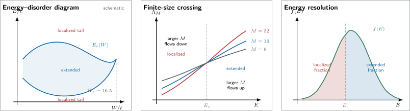
Three ledgers for a mobility-edge claim. Left: a schematic simple-cubic $E$–$W$ diagram has localized spectral tails surrounding an extended core that collapses near the band-center threshold; the curve is qualitative, not a numerical phase boundary. Center: the renormalized quasi-one-dimensional localization length $\Lambda_M$ decreases with width on the localized side, increases on the extended side, and is scale-invariant at $E_c$ up to corrections. Right: an experimental energy distribution $f(E)$ that straddles $E_c$ necessarily mixes localized and extended fractions.

Why three dimensions permit the transition

For a hypercubic conductor with bulk conductivity $\sigma$, the dimensionless conductance scales classically as

$$g(L) \sim \frac{ \sigma L^{d-2} }{ e^2/h }.$$

The geometric factor grows with $L$ in $d=3$, while localization corrections reduce conductance. Their competition permits an unstable critical point. On one side, the flow approaches a metal; on the other, it approaches exponentially small conductance.

This argument explains why a transition is possible, not where $E_c(W)$ lies. The edge location requires microscopic calculation or measurement. Spatial correlations in a laser speckle, long-range hopping, anisotropy, multiple orbitals, and magnetic fields can shift the edge strongly without changing every universal exponent.

Disorder broadening is not delocalization

The operator spectrum for bounded box disorder lies within the broad bound

$$-6t-\frac{W}{2} \le E \le 6t+\frac{W}{2}.$$

This growing spectral support does not imply a growing extended band. Disorder can add localized tail states while the extended region shrinks. A density-of-states plot can therefore broaden at the same time that the mobility window narrows.

That distinction is especially important in amorphous semiconductors and impurity bands. A spectroscopic onset locates available states; a transport onset locates states that participate in long-range motion under the stated conditions. Their separation is a mobility-tail regime, not automatically a clean band gap.

Critical Behavior

Diverging length

Choose a dimensionless tuning variable $\delta$ with $\delta=0$ at the edge and $\delta>0$ on the extended side. For an energy scan at fixed disorder, one convenient local definition is

$$\delta = \frac{ E-E_c }{ E_0 },$$

with the sign reversed at an upper edge if needed. The critical length diverges as

$$\xi_\pm(\delta) = \xi_{0,\pm} \lvert\delta\rvert^{-\nu}.$$

On the localized side, $\xi_-$ is the localization length. On the metallic side, $\xi_+$ is a correlation or crossover length beyond which metallic scaling is established. The amplitudes $\xi_{0,+}$ and $\xi_{0,-}$ need not be equal.

For the three-dimensional orthogonal class, a high-precision transfer-matrix benchmark is

$$\nu \simeq 1.571,$$

with a reported interval approximately

$$1.563 \le \nu \le 1.579.$$

The exponent is universal within the class; $W_c$, $E_c$, critical conductance distribution, and finite-size amplitudes generally are not. Multifractal finite-size scaling gives compatible values when correlations and irrelevant fields are treated carefully.

For disordered critical points, the finite-size correlation-length exponent is constrained by the Chayes bound

$$\nu_{\mathrm{FS}} \ge \frac{2}{d}.$$

The three-dimensional orthogonal value comfortably satisfies this bound. A fitted violation should trigger an audit of system sizes, disorder averaging, crossover scales, and the distinction between intrinsic and finite-size exponents.

Conductivity exponent

On the metallic side at zero temperature,

$$\sigma(\delta,0) \propto \delta^s.$$

Under noninteracting one-parameter scaling with a finite nonsingular density of states, the Wegner relation gives

$$s = (d-2)\nu.$$

Thus in three dimensions,

$$s = \nu.$$

This relation is not a license to fit an interacting finite-temperature material with one exponent. Electron–electron interactions, changing carrier density, finite $L_\phi$, and inhomogeneity can introduce extra scaling variables and alter the transport analysis.

At criticality, the finite-sample conductance can be scale-invariant while the bulk conductivity behaves as

$$\sigma(L) \sim \frac{e^2}{h} L^{2-d}.$$

In $d=3$, the thermodynamic dc conductivity at the critical point therefore vanishes even though the finite-size dimensionless conductance remains of order unity.

Dynamical scaling

A frequency or observation time supplies a finite length,

$$L_\omega \sim \omega^{-1/z}.$$

For the standard noninteracting Anderson transition with a regular density of states, the dynamical exponent is

$$z=d.$$

The critical ac conductivity then scales as

$$\sigma(\omega,E_c) \propto \omega^{(d-2)/d},$$

so the three-dimensional benchmark is

$$\sigma(\omega,E_c) \propto \omega^{1/3}.$$

Finite temperature, interactions, and probe coupling can change this simple dynamical ledger. The limit order must be stated:

$$\lim_{\omega\to0} \lim_{L\to\infty} \ne \lim_{L\to\infty} \lim_{\omega\to0}$$

for quantities sensitive to discrete levels and finite-size transport.

Critical eigenstates are multifractal

Critical states are neither uniformly extended nor exponentially localized. For lattice probabilities

$$\mu_i = \lvert\psi_i\rvert^2,$$

define generalized participation moments

$$P_q = \sum_i \mu_i^q.$$

At criticality,

$$P_q \propto L^{-\tau_q},$$

with

$$\tau_q = d(q-1) + \Delta_q.$$

The anomalous exponents $\Delta_q$ vanish for a perfectly uniform extended state but are nonzero at an Anderson critical point. For $q=2$,

$$P_2 \propto L^{-D_2}, \qquad 0<D_2<d.$$

Multifractality is a distributional statement over scales and disorder realizations. A single visually sparse eigenfunction is not a multifractal analysis.

Finite-Size Identification

Transfer-matrix crossing

For a long bar with transverse width $M$, let $\lambda_M(E)$ be the quasi-one-dimensional localization length obtained from the smallest positive Lyapunov exponent. The dimensionless ratio

$$\Lambda_M(E) = \frac{ \lambda_M(E) }{ M }$$

has a useful width dependence:

$$\begin{array}{c|c} \text{bulk regime} & \text{trend as }M\text{ increases} \\ \hline \text{localized} & \Lambda_M\text{ decreases} \\ \text{critical} & \Lambda_M\text{ is scale-invariant} \\ \text{extended} & \Lambda_M\text{ increases}. \end{array}$$

Near the edge, a precision fit uses both relevant and irrelevant scaling fields:

$$\Lambda_M = \mathcal F \left( \chi(\delta)M^{1/\nu}, \phi(\delta)M^y \right), \qquad y<0.$$

The irrelevant term explains why crossings of successive widths drift rather than meeting at one perfect point. If corrections are negligible, the critical slope obeys

$$\left. \frac{ \partial\Lambda_M }{ \partial E } \right|_{E_c} \propto M^{1/\nu}.$$

One crossing of two widths estimates a crossover. A mobility-edge result should vary the minimum width, polynomial order, energy window, irrelevant terms, random samples, and boundary conditions. Finite-Size Scaling in Numerics owns the general covariance and model-selection workflow.

Complementary observables

Observable	Localized side	Extended side	Critical behavior or warning
$\Lambda_M=\lambda_M/M$	decreases with $M$	increases with $M$	crossing with irrelevant drift
$P_2$	approaches a nonzero scale	$\sim L^{-d}$	$\sim L^{-D_2}$
Typical conductance	exponentially small	finite-size metallic flow	broad scale-invariant distribution
Level statistics	Poisson after symmetry resolution	Wigner–Dyson	intermediate, scale-invariant statistics
Boundary sensitivity	exponentially weak	comparable to level spacing	Thouless number of order unity
Typical local DOS	tends toward zero with resolution scaling	remains finite	broad multifractal distribution
Wave-packet width	saturates	diffusive or anomalous growth	finite-time critical scaling

Agreement among observables is stronger than any one crossing. Level statistics can be Poisson because of unresolved symmetries or integrability. A broadened local density of states can look finite in a localized phase. Conductance depends on leads and boundaries. Every estimator has a failure mode.

Energy bins and mixed states

Suppose a numerical bin has width $\Delta E$. The extracted observable is effectively

$$\overline{\mathcal O}_{\Delta E}(E) = \frac{1}{\Delta E} \int_{E-\Delta E/2}^{E+\Delta E/2} dE'\, \mathcal O(E').$$

If $\Delta E$ exceeds the critical window for the largest size, localized and extended states are pooled. The apparent crossing broadens and can drift. A defensible analysis reduces $\Delta E$, increases sample count to compensate, and checks that the result is stable.

Experimental Probes

Electronic materials

In a disordered electronic solid, the most direct control variable is often carrier density, gate voltage, pressure, composition, or magnetic field rather than eigenenergy itself. These knobs can simultaneously change:

• the chemical potential;
• disorder screening and correlation;
• carrier interactions;
• band structure and effective mass;
• inelastic scattering and sample homogeneity.

A density-tuned metal–insulator transition is therefore not automatically a clean scan of $\mu$ through a fixed single-particle $E_c$. The microscopic ensemble must remain sufficiently controlled for that interpretation.

Transport evidence is strongest when several regimes close quantitatively. If thermal activation reaches extended states, the fitted $\Delta_{\mathrm{mob}}$ should agree with an independently determined chemical-potential offset. If hopping dominates, its $T_0$, localization length, density of states, and dielectric scale should close as described on Anderson Insulators. Tunneling or photoemission can locate spectral weight, but spectral weight alone does not establish mobility.

The local density-of-states distribution is more informative than its average. For a resolution-broadened LDOS $\rho_i(E,\eta)$, compare

$$\rho_{\mathrm{av}}(E,\eta) = \left\langle \rho_i(E,\eta) \right\rangle$$

with

$$\rho_{\mathrm{typ}}(E,\eta) = \exp \left\langle \ln\rho_i(E,\eta) \right\rangle.$$

The typical value is strongly suppressed by localization while the average can remain finite because of rare peaks. The limits $\eta\to0$ and $L\to\infty$ must still be scaled; finite broadening can make every site appear weakly connected.

Ultracold atoms

Cold atoms offer unusually direct control over disorder and dynamics. A typical protocol prepares an energy distribution $f(E)$, releases the cloud into a three-dimensional random potential, and tracks expansion. If localized states lie below $E_c$, the ideal localized fraction is

$$f_{\mathrm{loc}} = \int_{-\infty}^{E_c} dE\, f(E).$$

The extended fraction is

$$f_{\mathrm{ext}} = 1-f_{\mathrm{loc}}.$$

This makes energy calibration central. An uncertainty in $f(E)$ or the zero of the speckle potential maps directly into uncertainty in $E_c$. Residual interactions, finite observation time, trap curvature, anisotropic speckle correlations, and classical trapping below a percolation threshold must be controlled.

Expansion data should separate at least three possibilities:

$$\begin{array}{c|c} \text{mechanism} & \text{long-time signature} \\ \hline \text{diffusion} & \Delta r^2(t)\propto t \\ \text{Anderson localization} & \Delta r^2(t)\text{ saturates quantum mechanically} \\ \text{classical trapping or loss} & \text{stationary density without localization scaling}. \end{array}$$

Three-dimensional speckle experiments have measured a disorder-dependent mobility edge, but comparison to theory requires the actual correlation tensor and energy distribution rather than an ideal white-noise model.

Classical waves

Frequency plays the role of energy for sound, microwaves, and light. A frequency scan can therefore map a mobility edge without Fermi occupation. The same conceptual distinction survives:

$$\text{nonzero mode density} \not\Rightarrow \text{extended transport}.$$

Absorption and out-of-plane leakage can also attenuate transmission exponentially. Time-resolved spreading, transverse confinement, delay statistics, sample-thickness scaling, and independent loss calibration are needed to distinguish localization from dissipation. Classical-wave experiments test the wave-interference universality class, not electron statistics or interaction physics.

Quantum Hall critical energies

In an ideal two-dimensional integer quantum Hall problem, disorder localizes most bulk states within a broadened Landau level while critical extended states mediate plateau transitions. Finite temperature and finite size broaden each critical energy into an apparent conducting interval.

This is a mobility-edge problem with topological structure. The Hall invariant, chiral boundary transport, and plateau-transition scaling are essential; importing the zero-field three-dimensional phase diagram is incorrect. Integer Quantum Hall Effect is the canonical home for that case.

Evidence ladder

1. Suggestive: transport or expansion changes rapidly with energy-like control.
2. Energy-resolved: localized and extended diagnostics are measured in declared energy windows.
3. Scale-discriminating: size, time, width, or frequency trends reverse across one boundary.
4. Critical: a common $E_c$ and $\nu$ survive corrections to scaling and fit-window changes.
5. Mechanism-level: disorder correlations, symmetry, interactions, energy resolution, loss, heating, and classical trapping are independently controlled.

Common Mistakes

• Calling a density-of-states onset a mobility edge.
• Treating a mobility gap as a spectral gap.
• Quoting $E_c$ without the disorder distribution, correlation length, symmetry class, and energy zero.
• Declaring finite eigenstates “extended” from a large participation ratio without size scaling.
• Pooling localized and extended states in one energy bin.
• Inferring an edge from one crossing of two small widths.
• Omitting irrelevant scaling fields when crossings drift systematically.
• Treating $W_c/t\simeq16.53$ as universal beyond the simple-cubic box-disorder benchmark.
• Assuming every one-dimensional or two-dimensional disordered model has an ordinary mobility edge.
• Calling an Arrhenius transport scale $\Delta_{\mathrm{mob}}$ without excluding a band gap, contact barrier, polaron, or nearest-neighbor hop.
• Changing doping and claiming a pure energy scan while disorder and interactions also change.
• Mistaking absorption, leakage, finite observation time, or classical trapping for wave localization.
• Equating a single-particle mobility edge with a many-body mobility edge.
• Ignoring the order of the $L\to\infty$, $\omega\to0$, $T\to0$, and resolution limits.

Exercises

1. Spectral edge, mobility edge, and mobility gap

A model has $\rho(E)>0$ for $-5t<E<5t$. States are localized for $-5t<E<-2t$ and $2t<E<5t$, and extended for $-2t<E<2t$. Identify the spectral edges, mobility edges, and any mobility gaps.

Solution

The spectral edges are

$$E_{\mathrm s}^{(-)} = -5t, \qquad E_{\mathrm s}^{(+)} = 5t.$$

The mobility edges are

$$E_c^{(-)} = -2t, \qquad E_c^{(+)} = 2t.$$

The intervals

$$(-5t,-2t) \qquad\text{and}\qquad (2t,5t)$$

contain states but no extended states, so both are mobility-gap intervals and, more specifically, localized spectral tails. When “the mobility gap” refers to transport at a specified chemical potential, one must also state which interval contains $\mu$.

2. Band-center benchmark

For the simple-cubic box-disorder Anderson model at $E=0$, classify $W=12t$ and $W=18t$ using $W_c\simeq16.53t$. What does this classification not prove?

Solution

At the thermodynamic, noninteracting, orthogonal-class benchmark,

$$12t < W_c$$

places the band-center state on the extended side, while

$$18t > W_c$$

places it on the localized side.

This comparison does not classify other energies, disorder distributions, correlated disorder, finite samples, interacting materials, or a different symmetry class. It also does not prove that a sample of available size has reached its asymptotic regime.

3. Critical length scale

Take

$$\xi(\delta) = 2a \lvert\delta\rvert^{-1.571}.$$

Estimate $\xi/a$ at $\lvert\delta\rvert=0.020$. What minimum system-size lesson follows?

Solution

Substitution gives

$$\frac{\xi}{a} = 2 \times (0.020)^{-1.571} \simeq 9.33\times10^2.$$

A system with $L\ll900a$ cannot resolve the asymptotic side of the transition at this detuning. It will lie in a broad critical crossover and must be analyzed by finite-size scaling rather than by a localized-versus-extended snapshot.

4. Slope scaling

If irrelevant corrections are negligible, the transfer-matrix crossing slope scales as $M^{1/\nu}$. For $\nu=1.571$, what is the slope ratio between widths $M=48$ and $M=12$? Conversely, what $\nu$ follows from a measured ratio $2.42$?

Solution

The predicted ratio is

$$\frac{S_{48}}{S_{12}} = \left( \frac{48}{12} \right)^{1/1.571} = 4^{1/1.571} \simeq 2.42.$$

Inverting the relation,

$$\nu = \frac{\ln(48/12)}{\ln(2.42)} \simeq 1.57.$$

A real fit should include correlated uncertainties and test irrelevant-field corrections rather than infer $\nu$ from only two widths.

5. Wegner conductivity exponent

Use one-parameter scaling in $d=3$ with $\nu=1.571$. Find $s$ and estimate $\sigma/\sigma_\ast$ at $\delta=0.030$ if

$$\sigma = \sigma_\ast \delta^s.$$

Solution

The Wegner relation gives

$$s = (3-2)\nu = 1.571.$$

Therefore

$$\frac{\sigma}{\sigma_\ast} = (0.030)^{1.571} \simeq 4.05\times10^{-3}.$$

The small value illustrates how a state can be on the extended side yet have a very small asymptotic conductivity close to the edge.

6. Participation-ratio scaling

When $L$ doubles in $d=3$, find the expected ratio $P_2(2L)/P_2(L)$ for a uniform extended state, a localized state, and a critical state with $D_2=1.3$.

Solution

For a uniform extended state,

$$\frac{P_2(2L)}{P_2(L)} = 2^{-3} = \frac18.$$

For a localized state much smaller than both samples,

$$\frac{P_2(2L)}{P_2(L)} \simeq 1.$$

For the critical state,

$$\frac{P_2(2L)}{P_2(L)} = 2^{-1.3} \simeq 0.406.$$

The intermediate scaling is the multifractal signature; the numerical value $D_2=1.3$ is illustrative and class-dependent.

7. Finite energy resolution

An atomic ensemble has a Gaussian energy distribution with mean

$$E_0 = E_c+0.5\Delta$$

and standard deviation $\Delta$. States with $E<E_c$ are localized. What localized fraction is present before any dynamical imperfection?

Solution

Standardizing the Gaussian,

$$z_c = \frac{ E_c-E_0 }{ \Delta } = -0.5.$$

Hence

$$f_{\mathrm{loc}} = \Phi(-0.5) \simeq 0.3085,$$

where $\Phi$ is the standard normal cumulative distribution. Almost $31\%$ of the ensemble is localized even though the mean energy lies above the edge. A sharp threshold cannot be read directly from the mean.

8. Audit a mobility-edge claim

A simulation reports a mobility edge from an IPR color map for one size, and an experiment reports the same edge from exponentially decaying transmission at one sample thickness. List at least eight missing checks.

Solution

A strong audit should require:

1. several system sizes and a declared thermodynamic scaling form;
2. narrower and shifted energy bins;
3. disorder-realization counts and distributional uncertainties;
4. an independent observable such as transfer length, conductance, level statistics, or wave-packet spreading;
5. resolved symmetries and degeneracies;
6. irrelevant-field and fit-window stability tests;
7. disorder distribution, correlation tensor, energy zero, and boundary conditions;
8. loss and absorption calibration for the transmission experiment;
9. thickness and transverse-size scaling;
10. finite-time, finite-frequency, and instrumental-resolution tests;
11. controls against classical trapping or forbidden propagation;
12. interactions, dephasing, heating, and inhomogeneity estimates.

The two observations may be compatible with one mobility edge, but neither establishes it at mechanism level on its own.

Connections

• Anderson Localization owns the random Hamiltonian, exponential localization, transfer matrices, participation ratios, and direct diagnostics.
• Scaling Theory of Localization derives the conductance beta function, critical fixed point, Wegner relation, and nonlinear-sigma-model bridge.
• Anderson Insulators treats activation, Mott variable-range hopping, Coulomb gaps, and Efros–Shklovskii transport on the localized side.
• Random Matrix Theory in Quantum Matter supplies the unfolded Poisson and Wigner–Dyson baselines against which critical level statistics are compared.
• Disorder in Quantum Matter defines random-potential ensembles, spatial correlators, scattering times, and disorder-control standards.
• Finite-Size Scaling in Numerics develops covariance-aware crossings, irrelevant corrections, collapse tests, and uncertainty reporting.
• Density of States owns spectral state counting and van Hove structure, which must not be confused with mobility.
• Spectral Functions separates spectral weight, linewidth, quasiparticle residue, and measured intensity from spatial extension.
• Quantum Coherence in Conductors owns dephasing, thermal averaging, escape, and the finite lengths that truncate localization flow.
• Integer Quantum Hall Effect develops topological critical energies, localized bulk states, chiral edges, and plateau-transition evidence.
• Many-Body Localization Preview distinguishes a single-particle energy edge from interacting finite-energy-density localization and its stability questions.

References

1. P. W. Anderson, “Absence of Diffusion in Certain Random Lattices,” Physical Review 109, 1492–1505 (1958), doi:10.1103/PhysRev.109.1492. Establishes disorder-induced absence of diffusion in the benchmark random lattice.
2. N. F. Mott, “Electrons in Disordered Structures,” Advances in Physics 16, 49–144 (1967), doi:10.1080/00018736700101265. Develops the mobility-edge concept for disordered electronic systems.
3. J. T. Edwards and D. J. Thouless, “Numerical Studies of Localization in Disordered Systems,” Journal of Physics C: Solid State Physics 5, 807–820 (1972), doi:10.1088/0022-3719/5/8/007. Introduces boundary-condition sensitivity as an energy-resolved localization criterion.
4. D. J. Thouless, “Electrons in Disordered Systems and the Theory of Localization,” Physics Reports 13, 93–142 (1974), doi:10.1016/0370-1573(74)90029-5. Connects spectral sensitivity, diffusion, and localization scales.
5. F. J. Wegner, “Electrons in Disordered Systems. Scaling near the Mobility Edge,” Zeitschrift für Physik B 25, 327–337 (1976), doi:10.1007/BF01315248. Derives critical scaling relations near a mobility edge.
6. E. Abrahams, P. W. Anderson, D. C. Licciardello, and T. V. Ramakrishnan, “Scaling Theory of Localization: Absence of Quantum Diffusion in Two Dimensions,” Physical Review Letters 42, 673–676 (1979), doi:10.1103/PhysRevLett.42.673. Establishes one-parameter conductance flow and the three-dimensional unstable fixed point.
7. A. MacKinnon and B. Kramer, “One-Parameter Scaling of Localization Length and Conductance in Disordered Systems,” Physical Review Letters 47, 1546–1549 (1981), doi:10.1103/PhysRevLett.47.1546. Introduces recursive transfer-matrix finite-size scaling.
8. A. MacKinnon and B. Kramer, “The Scaling Theory of Electrons in Disordered Solids: Additional Numerical Results,” Zeitschrift für Physik B 53, 1–13 (1983), doi:10.1007/BF01578242. Maps dimensional and energy-dependent localization with quasi-one-dimensional bars.
9. J. T. Chayes, L. Chayes, D. S. Fisher, and T. Spencer, “Finite-Size Scaling and Correlation Lengths for Disordered Systems,” Physical Review Letters 57, 2999–3002 (1986), doi:10.1103/PhysRevLett.57.2999. Establishes the disorder-sensitive finite-size correlation-length bound.
10. K. Slevin and T. Ohtsuki, “Corrections to Scaling at the Anderson Transition,” Physical Review Letters 82, 382–385 (1999), doi:10.1103/PhysRevLett.82.382. Shows why irrelevant scaling fields are needed for precision crossings.
11. F. Evers and A. D. Mirlin, “Anderson Transitions,” Reviews of Modern Physics 80, 1355–1417 (2008), doi:10.1103/RevModPhys.80.1355. Reviews universality classes, multifractality, critical statistics, and field theory.
12. G. Schubert, J. Schleede, K. Byczuk, H. Fehske, and D. Vollhardt, “Distribution of the Local Density of States as a Criterion for Anderson Localization,” Physical Review B 81, 155106 (2010), doi:10.1103/PhysRevB.81.155106. Develops finite-size and distributional LDOS diagnostics.
13. A. Rodriguez, L. J. Vasquez, K. Slevin, and R. A. Römer, “Multifractal Finite-Size Scaling and Universality at the Anderson Transition,” Physical Review B 84, 134209 (2011), doi:10.1103/PhysRevB.84.134209. Provides covariance-aware multifractal estimates of $W_c$, $\nu$, and anomalous exponents.
14. F. Jendrzejewski, A. Bernard, K. Müller, et al., “Three-Dimensional Localization of Ultracold Atoms in an Optical Disordered Potential,” Nature Physics 8, 398–403 (2012), doi:10.1038/nphys2256. Separates localized and diffusive components in three-dimensional speckle disorder.
15. K. Slevin and T. Ohtsuki, “Critical Exponent for the Anderson Transition in the Three-Dimensional Orthogonal Universality Class,” New Journal of Physics 16, 015012 (2014), doi:10.1088/1367-2630/16/1/015012. Tests exponent universality across box, normal, and Cauchy disorder.
16. G. Semeghini, M. Landini, P. Castilho, et al., “Measurement of the Mobility Edge for 3D Anderson Localization,” Nature Physics 11, 554–559 (2015), doi:10.1038/nphys3339. Measures the disorder–energy boundary with controlled atomic matter waves.
17. E. Fratini and S. Pilati, “Anderson Localization of Matter Waves in Quantum-Chaos Theory,” Physical Review A 91, 061601(R) (2015), doi:10.1103/PhysRevA.91.061601. Quantifies how realistic anisotropic speckle correlations shift the mobility edge.
18. A. Yamilov, H. Cao, and S. E. Skipetrov, “Anderson Transition for Light in a Three-Dimensional Random Medium,” Physical Review Letters 134, 046302 (2025), doi:10.1103/PhysRevLett.134.046302. Tests mobility-edge scaling and critical transmission statistics for electromagnetic waves.

Further Reading

• B. Kramer and A. MacKinnon, “Localization: Theory and Experiment,” Reports on Progress in Physics 56, 1469–1564 (1993), doi:10.1088/0034-4885/56/12/001. A broad bridge among models, scaling methods, and material experiments.
• E. Akkermans and G. Montambaux, Mesoscopic Physics of Electrons and Photons, Cambridge University Press, 2007. A path-interference and transport treatment of diffusion through localization.
• K. B. Efetov, Supersymmetry in Disorder and Chaos, Cambridge University Press, 1997. A technical nonlinear-sigma-model account of Anderson criticality.