Density of States

The density of states counts independent one-particle states per unit energy. For crystalline bands it compresses the full dispersion $\varepsilon_n(\mathbf k)$ into an energy distribution, retaining how much state space lies near each energy while discarding where those states occur in momentum space.

That compression is powerful but incomplete. The density of states controls filling integrals, low-temperature thermodynamics, phase space for transitions, and many spectroscopic line shapes. It does not by itself determine velocities, scattering times, optical matrix elements, topology, or whether states are extended.

This page is the canonical home for the band density of states in quantum matter: Brillouin-zone counting, normalization per cell and per volume, dimensional threshold laws, van Hove singularities, tight-binding examples, projected and local variants, thermodynamic use, spectroscopy, and numerical evaluation. Density of States: First Encounter owns the free-particle continuum derivation, Green Functions and Density of States owns the resolvent formulation, and Density of States in Transition Rates owns final-state phase space.

Required background. Brillouin Zones supplies the full-zone measure and state-counting domain; Density of States: First Encounter supplies the continuum counting and delta-function definition generalized here to bands.

Definition

For a finite one-particle spectrum,

$$D(E) = \sum_{\lambda} \delta(E-E_{\lambda}).$$

$D(E)$ is a distribution with units of inverse energy. The label $\lambda$ must enumerate every independent state exactly once, including any spin, valley, orbital, or other degeneracy intended by the convention.

The integrated density of states is

$$\mathcal N(E) = \int_{-\infty}^{E} dE'\, D(E').$$

For a finite system it is a staircase that jumps by the degeneracy of each level. Distributionally,

$$D(E) = \frac{d\mathcal N}{dE}.$$

A smooth curve appears only after a thermodynamic limit, a coarse graining, or an explicitly stated broadening.

Normalization Ledger

Three normalizations are common and must not be mixed.

Total density

For $N_c$ cells,

$$D_{\mathrm{tot}}(E) = \sum_{n,\mathbf k} \delta \left[ E-\varepsilon_n(\mathbf k) \right].$$

It scales extensively with system size.

Density per primitive cell

Define

$$\rho_c(E) = \frac{D_{\mathrm{tot}}(E)}{N_c}.$$

For a model with $N_b$ bands, where $n$ already includes all counted internal states,

$$\int_{-\infty}^{\infty} dE\, \rho_c(E) = N_b.$$

Thus $\rho_c$ has units of states per cell per energy.

Density per physical volume

With $V=N_c\Omega_c$,

$$\rho_V(E) = \frac{D_{\mathrm{tot}}(E)}{V} = \frac{\rho_c(E)}{\Omega_c}.$$

Its units are states per physical volume per energy. In two-dimensional materials one often quotes density per area; in one dimension, per length.

If a displayed band structure omits spin and every band is spin degenerate, multiply by $g_s=2$ only once. When spin–orbit coupling splits the bands and spin is already included in $n$, no additional factor is allowed.

Counting States in the Brillouin Zone

For a finite periodic crystal,

$$\rho_c(E) = \frac{1}{N_c} \sum_{n,\mathbf k} \delta \left[ E-\varepsilon_n(\mathbf k) \right].$$

The thermodynamic rule

$$\frac{1}{N_c} \sum_{\mathbf k} \longrightarrow \frac{\Omega_c}{(2\pi)^d} \int_{\mathrm{BZ}} d^dk$$

gives

$$\rho_c(E) = \frac{\Omega_c}{(2\pi)^d} \sum_n \int_{\mathrm{BZ}} d^dk\, \delta \left[ E-\varepsilon_n(\mathbf k) \right].$$

Equivalently,

$$\rho_V(E) = \frac{1}{(2\pi)^d} \sum_n \int_{\mathrm{BZ}} d^dk\, \delta \left[ E-\varepsilon_n(\mathbf k) \right].$$

The Brillouin-zone volume

$$\operatorname{Vol}(\mathrm{BZ}) = \frac{(2\pi)^d}{\Omega_c}$$

immediately proves the band-count sum rule.

Integrated form

The number of states per cell below $E$ is

$$\mathcal N_c(E) = \frac{\Omega_c}{(2\pi)^d} \sum_n \int_{\mathrm{BZ}} d^dk\, \Theta \left[ E-\varepsilon_n(\mathbf k) \right].$$

This is the Brillouin-zone volume occupied by all sublevel sets $\varepsilon_n(\mathbf k)\leq E$, measured in units of one state per band per cell.

Constant-Energy Geometry

Away from critical points, the delta-function integral can be converted into an integral over the constant-energy surface

$$\mathcal S_n(E) = \left\{ \mathbf k: \varepsilon_n(\mathbf k)=E \right\}.$$

The coarea formula gives

$$\rho_V(E) = \frac{1}{(2\pi)^d} \sum_n \int_{\mathcal S_n(E)} \frac{ dS_{\mathbf k} }{ \left| \boldsymbol\nabla_{\mathbf k} \varepsilon_n(\mathbf k) \right| }.$$

Using

$$\mathbf v_n(\mathbf k) = \frac{1}{\hbar} \boldsymbol\nabla_{\mathbf k} \varepsilon_n(\mathbf k),$$

this becomes

$$\rho_V(E) = \frac{1}{(2\pi)^d} \sum_n \int_{\mathcal S_n(E)} \frac{ dS_{\mathbf k} }{ \hbar|\mathbf v_n(\mathbf k)| }.$$

Large constant-energy surfaces and small group velocities both enhance the density of states. The formula is not regular at a critical point where $\boldsymbol\nabla_{\mathbf k}\varepsilon_n=\mathbf0$; those points generate van Hove nonanalyticities.

In one dimension, a constant-energy surface is a collection of roots $k_i$:

$$\rho_c(E) = \frac{a}{2\pi} \sum_{n,k_i} \frac{1}{ \left| d\varepsilon_n/dk \right|_{k_i} },$$

for a primitive length $a$. Each root must be counted, including symmetry-related left- and right-moving states.

Parabolic Band Edges

Consider an isotropic extremum

$$\varepsilon(\mathbf k) = E_0 + \frac{\hbar^2k^2}{2m^\ast}, \qquad m^\ast>0,$$

with total internal degeneracy $g$. Define

$$\xi = E-E_0.$$

The number of states per volume below $E$ is

$$\frac{\mathcal N(E)}{V} = g \frac{S_{d-1}}{ d(2\pi)^d } \left( \frac{2m^\ast\xi}{\hbar^2} \right)^{d/2} \Theta(\xi),$$

where

$$S_{d-1} = \frac{ 2\pi^{d/2} }{ \Gamma(d/2) }$$

is the area of the unit $(d-1)$-sphere. Differentiation gives

$$\rho_d(E) = g \frac{S_{d-1}}{(2\pi)^d} \frac{m^\ast}{\hbar^2} \left( \frac{2m^\ast\xi}{\hbar^2} \right)^{(d-2)/2} \Theta(\xi).$$

The threshold law is therefore

$$\rho_d(E) \propto \xi^{d/2-1} \Theta(\xi).$$

One dimension

$$\rho_1(E) = \frac{g}{\pi\hbar} \sqrt{ \frac{m^\ast}{2\xi} } \Theta(\xi).$$

The inverse-square-root divergence reflects the vanishing velocity at the band edge.

Two dimensions

$$\rho_2(E) = \frac{g m^\ast}{2\pi\hbar^2} \Theta(\xi).$$

An ideal parabolic two-dimensional band has a constant density of states with a step at its edge.

Three dimensions

$$\rho_3(E) = \frac{g}{4\pi^2} \left( \frac{2m^\ast}{\hbar^2} \right)^{3/2} \sqrt{\xi} \, \Theta(\xi).$$

The density rises continuously with a square-root onset.

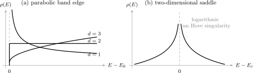
Dimensionality fixes the ideal threshold law near a nondegenerate parabolic minimum: divergence in $d=1$, a step in $d=2$, and a square-root onset in $d=3$. A nondegenerate saddle in two dimensions instead produces a logarithmic van Hove singularity. Disorder, interactions, finite temperature, and numerical broadening round these ideal features.

Van Hove Singularities

A van Hove critical point satisfies

$$\boldsymbol\nabla_{\mathbf k} \varepsilon_n(\mathbf k_c) = \mathbf0.$$

Near an isolated nondegenerate critical point,

$$\varepsilon_n(\mathbf k_c+\mathbf q) = E_c + \frac12 \mathbf q^{\mathsf T} \mathcal H \mathbf q + O(q^3),$$

where $\mathcal H$ is the Hessian matrix of second derivatives. The numbers of positive and negative Hessian eigenvalues distinguish minima, maxima, and saddles.

For ordinary Morse critical points:

• one-dimensional extrema produce inverse-square-root divergences;
• two-dimensional extrema produce step discontinuities;
• two-dimensional saddles produce logarithmic divergences;
• three-dimensional extrema produce square-root onsets;
• three-dimensional saddles generally produce finite square-root cusps with a singular derivative.

At a two-dimensional saddle,

$$\varepsilon-E_c \approx \alpha q_x^2 - \beta q_y^2, \qquad \alpha,\beta>0.$$

With a finite momentum cutoff $\Lambda$ set by the range of the local expansion,

$$\rho_{\mathrm{sing}}(E) \sim C \ln \left( \frac{\Lambda_E}{ |E-E_c| } \right),$$

where $C>0$ depends on the curvature and normalization. The logarithm is universal; its additive constant and ultraviolet scale are not.

Beyond ordinary critical points

A flat band, a line of stationary points, or a critical point with a singular Hessian can produce stronger or nonstandard behavior. Such higher-order van Hove singularities require their own local expansion rather than the quadratic Morse classification.

Symmetry can enforce several equivalent critical points at the same energy, multiplying the singular contribution. Conversely, spin–orbit coupling, strain, or symmetry breaking can split one feature into several nearby peaks.

Example: One-Dimensional Tight-Binding Band

For

$$\varepsilon(k) = \epsilon_0 - 2t\cos(ka),$$

the spinless density per cell is

$$\rho_c(E) = \frac{ \Theta \left( 2|t|-|E-\epsilon_0| \right) }{ \pi \sqrt{ 4t^2-(E-\epsilon_0)^2 } }.$$

It diverges at both band edges,

$$E = \epsilon_0\pm2|t|,$$

and obeys

$$\int dE\, \rho_c(E) = 1.$$

The singularities do not represent extra states. They describe the compression of a fixed number of $k$ states into a narrow energy interval where $d\varepsilon/dk$ vanishes.

Example: Square-Lattice Saddle

For nearest-neighbor hopping,

$$\varepsilon(\mathbf k) = -2t \left[ \cos(k_xa) + \cos(k_ya) \right].$$

The saddle points at $(\pi/a,0)$ and $(0,\pi/a)$ have energy $E_c=0$. The exact spinless density per cell can be written

$$\rho_c(E) = \frac{ \Theta(4|t|-|E|) }{ 2\pi^2|t| } K \left[ 1- \left( \frac{E}{4t} \right)^2 \right],$$

where the complete elliptic integral is defined by

$$K(m) = \int_0^{\pi/2} \frac{d\theta}{ \sqrt{ 1-m\sin^2\theta } }.$$

$K(m)$ diverges logarithmically as $m\to1$, giving the van Hove singularity at $E=0$. At the band edges $E=\pm4|t|$, the density approaches the finite two-dimensional parabolic-edge value.

Example: Two-Dimensional Dirac Cone

For one isotropic cone,

$$\varepsilon_{\pm}(\mathbf q) = \pm\hbar v|\mathbf q|,$$

the density per area, including a declared degeneracy $g$, is

$$\rho_A(E) = \frac{ g|E| }{ 2\pi\hbar^2v^2 }.$$

It vanishes linearly at the node. A zero density at one energy does not imply a finite band gap: a Dirac semimetal has states arbitrarily close to the nodal energy.

Flat and Nearly Flat Bands

An exactly flat band with $w$ states per cell at $E_f$ contributes

$$\rho_c^{\mathrm{flat}}(E) = w\delta(E-E_f).$$

A small bandwidth spreads this weight into a large but finite peak. Interactions and disorder can qualitatively reorganize a partially filled flat band, so the noninteracting density alone cannot determine the resulting phase.

Projected and Local Densities

For normalized Bloch eigenvectors in an orthonormal orbital basis, the orbital-projected density per cell is

$$\rho_{\alpha}(E) = \frac{1}{N_c} \sum_{n,\mathbf k} \left| u_{n\alpha}(\mathbf k) \right|^2 \delta \left[ E-\varepsilon_n(\mathbf k) \right].$$

Completeness gives

$$\sum_{\alpha} \rho_{\alpha}(E) = \rho_c(E).$$

Individual orbital projections depend on the retained basis and on unitary rotations among orbitals. They are useful diagnostics, not basis-independent observables.

The real-space local density of states is

$$\rho(\mathbf r,E) = \sum_{\lambda} \left| \psi_{\lambda}(\mathbf r) \right|^2 \delta(E-E_{\lambda}).$$

It resolves surfaces, defects, sublattices, and orbital texture. Integrating over the sample returns the total density of states.

Green Functions and Interactions

For a one-particle or quasiparticle retarded Green function,

$$\rho(E) = -\frac{1}{\pi} \operatorname{Im} \operatorname{Tr} G^R(E),$$

with the trace and normalization chosen for total, local, or per-cell density. In a noninteracting band model, poles reproduce delta functions. Interactions and disorder can shift poles, reduce quasiparticle weight, and create incoherent continua.

The resulting single-particle spectral density is not the many-body level density

$$\sum_m \delta(E-E_m^{\mathrm{many-body}}),$$

which counts entire many-body eigenstates and has very different scaling. Spectral Functions and Green Functions and Density of States develop that distinction.

Filling and Thermodynamics

For fermions, the particle number per cell is

$$\nu(T,\mu) = \int_{-\infty}^{\infty} dE\, \rho_c(E) f(E-\mu),$$

where

$$f(E-\mu) = \frac{1}{ e^{(E-\mu)/(k_{\mathrm B}T)} +1 }.$$

At zero temperature,

$$\nu(0,\mu) = \mathcal N_c(\mu).$$

The internal energy per volume of a noninteracting band system is

$$\frac{U}{V} = \int dE\, E \rho_V(E) f(E-\mu).$$

If $\rho_V(E)$ is smooth on the scale $k_{\mathrm B}T$ around the Fermi energy,

$$\frac{C_V}{V} = \frac{\pi^2}{3} k_{\mathrm B}^2 T \rho_V(E_{\mathrm F}) + O(T^3).$$

This linear coefficient measures the quasiparticle density of states in a Fermi liquid, including interaction renormalization. A nearby van Hove singularity or narrow band can invalidate the assumption of a locally smooth density.

The density of states is not an occupation function. Empty and filled states contribute equally to $\rho$; occupation enters through $f$, a Bose factor, or a nonequilibrium distribution.

Spectroscopy and Response

Tunneling

Under restrictive assumptions of weak tunneling, slowly varying matrix elements, and a featureless counterelectrode,

$$\frac{dI}{dV}$$

tracks a thermally broadened local density of states near energy $eV$. Tip orbital symmetry, barrier transmission, temperature, and many-body tunneling effects can reshape the signal.

Photoemission

Angle-resolved photoemission measures an occupied, matrix-element-weighted spectral function,

$$I(\mathbf k,\omega) \propto |M(\mathbf k,\omega)|^2 f(\omega) A(\mathbf k,\omega),$$

not the bare density of states. Momentum integration can resemble an occupied spectral density only after accounting for matrix elements and resolution.

Optical absorption

The joint density of states contains pairs of bands separated by photon energy:

$$J(\hbar\omega) = \sum_{n,m} \int_{\mathrm{BZ}} \frac{d^dk}{(2\pi)^d} \left[ f_n(\mathbf k)-f_m(\mathbf k) \right] \delta \left[ \varepsilon_m(\mathbf k) - \varepsilon_n(\mathbf k) - \hbar\omega \right].$$

It supplies phase space, but optical intensity also requires polarization-dependent transition matrix elements and selection rules. A peak in $J$ need not appear in a forbidden optical channel.

Transport

Conductivity is not determined by $\rho(E_{\mathrm F})$ alone. It weights states by velocity, scattering, and sometimes geometric factors. A large density caused by very flat states can coexist with poor charge transport.

Numerical Evaluation

Histogram

Sample $\varepsilon_n(\mathbf k)$ on a mesh and count states in energy bins. The result depends on bin width and can miss narrow or singular features unless the mesh is converged.

Explicit broadening

Replace each delta function by a normalized kernel. A Gaussian choice is

$$\delta_{\eta}^{\mathrm G}(x) = \frac{1}{ \eta\sqrt{\pi} } e^{-x^2/\eta^2},$$

while a Lorentzian is

$$\delta_{\eta}^{\mathrm L}(x) = \frac{1}{\pi} \frac{\eta}{ x^2+\eta^2 }.$$

The width $\eta$ is part of the result and must be reported. Gaussian instrumental resolution and Lorentzian lifetime broadening have different physical interpretations.

Interpolation methods

Tetrahedron and related simplex methods interpolate bands within momentum-space cells and integrate the delta function analytically. Adaptive meshes focus resolution near band extrema, crossings, and critical points. Wannier interpolation can cheaply generate dense meshes when its band subspace is validated.

Band Structure Workflows owns convergence and provenance of the crystal calculation and band data fed to these integrators. This page owns the normalized density-of-states estimator, its resolution controls, and its state-counting checks.

Sum-rule checks

Every numerical density should satisfy

$$\int dE\, \rho_c(E) = N_b$$

to numerical tolerance. A useful first moment is

$$\begin{aligned} \int dE\, E\rho_c(E) &= \frac{1}{N_c} \sum_{\mathbf k} \operatorname{Tr} h(\mathbf k) \\ &= \operatorname{Tr} t(\mathbf0), \end{aligned}$$

for a complete orthonormal tight-binding basis in the cell convention. Failure indicates missing weights, an energy-window cutoff, or inconsistent normalization.

Common Mistakes

Omitting the normalization label

“DOS” can mean total, per cell, per mole, per area, per volume, per spin, or spin summed. Units and degeneracies must be printed with the result.

Confusing density with occupation

$\rho(E)$ counts available states. The occupied density is $\rho(E)f(E-\mu)$ in equilibrium.

Using the surface formula at a critical point

$1/|\boldsymbol\nabla_{\mathbf k}\varepsilon|$ signals a singular limit. Analyze the local dispersion or retain the delta-function integral.

Interpreting broadening as intrinsic

A numerical $\eta$, instrumental resolution, disorder width, and many-body lifetime are different mechanisms. Do not exchange them silently.

Reading a projected density as unique

Orbital projections depend on basis and projector definitions. Total spectral weight and explicitly measurable matrix-element-weighted signals are more invariant.

Inferring transport from a large peak

Flat states raise the density but suppress velocity. Transport needs a velocity- and lifetime-weighted integral.

Confusing one-particle and many-body densities

The electronic band density counts addition or removal states in a one-particle description. It is not the exponentially large density of many-body energy eigenstates.

Exercises

Exercise 1: band-count sum rule

Starting from the Brillouin-zone expression for $\rho_c(E)$, prove that $N_b$ complete bands contribute $N_b$ states per cell.

Solution

Integrate over energy:

$$\begin{aligned} \int dE\, \rho_c(E) &= \frac{\Omega_c}{(2\pi)^d} \sum_{n=1}^{N_b} \int_{\mathrm{BZ}} d^dk \int dE\, \delta \left[ E-\varepsilon_n(\mathbf k) \right] \\ &= \frac{\Omega_c}{(2\pi)^d} N_b \operatorname{Vol}(\mathrm{BZ}). \end{aligned}$$

Since

$$\operatorname{Vol}(\mathrm{BZ}) = \frac{(2\pi)^d}{\Omega_c},$$

the result is $N_b$.

Exercise 2: dimensional threshold law

Derive the exponent of the density of states for

$$E-E_0 = A k^s, \qquad A>0,$$

in $d$ dimensions.

Solution

The number of states below energy $E$ is proportional to the volume of a $d$-ball of radius

$$k = \left( \frac{E-E_0}{A} \right)^{1/s}.$$

Therefore

$$\mathcal N(E) \propto (E-E_0)^{d/s} \Theta(E-E_0).$$

Differentiating,

$$\rho(E) \propto (E-E_0)^{d/s-1} \Theta(E-E_0).$$

The parabolic case has $s=2$, giving $d/2-1$. A two-dimensional Dirac cone has $s=1$, giving a linear density.

Exercise 3: one-dimensional chain

Derive the exact density per cell for

$$\varepsilon(k) = \epsilon_0-2t\cos(ka).$$

Solution

Use

$$\rho_c(E) = \frac{a}{2\pi} \int_{-\pi/a}^{\pi/a} dk\, \delta \left[ E-\epsilon_0+2t\cos(ka) \right].$$

Inside the band there are two roots with

$$\cos(ka) = -\frac{E-\epsilon_0}{2t}.$$

At either root,

$$\left| \frac{d\varepsilon}{dk} \right| = 2|t|a|\sin(ka)| = a \sqrt{ 4t^2-(E-\epsilon_0)^2 }.$$

Summing both roots gives

$$\rho_c(E) = \frac{ \Theta \left( 2|t|-|E-\epsilon_0| \right) }{ \pi \sqrt{ 4t^2-(E-\epsilon_0)^2 } }.$$

Exercise 4: logarithm from a saddle

Show qualitatively why

$$E-E_c = \alpha q_x^2-\beta q_y^2$$

produces a logarithmic density in two dimensions.

Solution

Rescale coordinates so the dispersion is

$$\xi = x^2-y^2.$$

Introduce

$$u = x+y, \qquad v = x-y,$$

so $\xi=uv$. Up to a constant Jacobian, the singular integral is

$$\int du\,dv\, \delta(\xi-uv).$$

Integrating over $v$ gives

$$\int \frac{du}{|u|}$$

over limits set by the local momentum cutoff and by $|uv|=|\xi|$. The result is

$$\rho_{\mathrm{sing}}(\xi) \propto \ln \left( \frac{\Lambda_E}{|\xi|} \right).$$

The cutoff fixes the nonsingular additive part, while the logarithmic dependence is universal for a nondegenerate two-dimensional saddle.

Exercise 5: projected sum rule

Prove that the sum of orbital-projected densities equals the total density in an orthonormal $N_{\mathrm{orb}}$-orbital model.

Solution

At each $(n,\mathbf k)$, eigenvector normalization gives

$$\sum_{\alpha=1}^{N_{\mathrm{orb}}} \left| u_{n\alpha}(\mathbf k) \right|^2 = 1.$$

Therefore

$$\begin{aligned} \sum_\alpha \rho_\alpha(E) &= \frac{1}{N_c} \sum_{n,\mathbf k} \sum_\alpha \left| u_{n\alpha}(\mathbf k) \right|^2 \delta \left[ E-\varepsilon_n(\mathbf k) \right] \\ &= \frac{1}{N_c} \sum_{n,\mathbf k} \delta \left[ E-\varepsilon_n(\mathbf k) \right] \\ &= \rho_c(E). \end{aligned}$$

For nonorthogonal orbitals, projector weights and the overlap metric must be defined explicitly.

Exercise 6: broadening preserves state count

Show that replacing every delta function by either normalized kernel given above preserves the integrated number of states.

Solution

Both kernels satisfy

$$\int_{-\infty}^{\infty} dx\, \delta_\eta(x) = 1.$$

For a broadened finite density,

$$D_\eta(E) = \sum_\lambda \delta_\eta(E-E_\lambda),$$

one has

$$\int dE\, D_\eta(E) = \sum_\lambda \int dE\, \delta_\eta(E-E_\lambda) = \sum_\lambda 1.$$

Broadening redistributes spectral weight in energy but must not create or remove total weight. A finite plotting window can appear to violate the rule by cutting off kernel tails.

Exercise 7: DOS is insufficient for conductivity

Construct two idealized bands with similar density of states near $E_{\mathrm F}$ but very different conductivities.

Solution

In a relaxation-time picture,

$$\sigma_{ij} \sim q^2 \sum_n \int \frac{d^dk}{(2\pi)^d} v_{n,i}(\mathbf k) v_{n,j}(\mathbf k) \tau_n(\mathbf k) \left( -\frac{\partial f}{\partial E} \right).$$

Two bands can have the same energy histogram and hence similar $\rho(E_{\mathrm F})$ while distributing their velocities differently. One may have nearly flat states with small $|\mathbf v|$, while the other has dispersive states and large velocity. Different scattering times can further separate their conductivities.

Thus density supplies state count but not the velocity and lifetime weights required for transport.

Connections

• The chapter gateway distinguishes energy-resolved state counting from Fermi-surface geometry and identifies the required dispersion and normalization data.
• Low-Dimensional Quantum Matter uses the parabolic band-edge law as one entry in a broader confinement, fluctuation, interaction, and dimensional-crossover ledger.
• Density of States formula card is the compact lookup for the counting and constant-energy-surface formulas.
• Density of States: First Encounter derives continuum free-particle state counting.
• Tight-Binding Models supplies the chain, square, and multiband dispersions used here.
• Fermi Surface applies the constant-energy-surface measure at the chemical potential and develops pockets, topology changes, and quantum oscillations.
• Itinerant Magnetism explains why a large Fermi-level density of states can enhance magnetic response but does not by itself determine the ordering wavevector or orbital channel.
• Stoner Criterion derives how the one-spin Fermi-level density of states controls the quadratic band cost of uniform polarization.
• BCS Theory uses an explicitly per-spin $N(0)$ in the pairing logarithm, condensation energy, and superconducting quasiparticle density of states.
• Effective Mass derives the geometric-mean density-of-states mass for anisotropic parabolic bands and keeps degeneracy factors separate.
• Green Functions and Density of States develops trace, local, and spectral representations.
• Mobility Edges explains why smooth spectral weight can cross a sharp localization boundary and how typical local density of states adds spatial information.
• Density of States in Transition Rates explains final-state phase space in Fermi’s golden rule.
• Sommerfeld Expansion derives low-temperature Fermi integrals when the density is smooth near the chemical potential.
• Spectral Functions treats interaction-broadened one-particle weight.

References

1. L. Van Hove, “The Occurrence of Singularities in the Elastic Frequency Distribution of a Crystal,” Physical Review 89, 1189–1193 (1953), doi:10.1103/PhysRev.89.1189.
2. N. W. Ashcroft and N. D. Mermin, Solid State Physics (Holt, Rinehart and Winston, 1976), Chapters 2, 8, and 12.
3. C. Kittel, Introduction to Solid State Physics, 8th ed. (Wiley, 2005), Chapters 6–8.
4. S. H. Simon, The Oxford Solid State Basics (Oxford University Press, 2013), Chapters 4–7.
5. M. P. Marder, Condensed Matter Physics, 2nd ed. (Wiley, 2010), Sections 6.3 and 7.2.
6. E. N. Economou, Green’s Functions in Quantum Physics, 3rd ed. (Springer, 2006), Chapters 1–3.
7. P. A. Lee, “Tight Binding and van Hove Singularity,” lecture notes for Theory of Solids I, MIT OpenCourseWare (2004), course materials.
8. G. Gilat and L. J. Raubenheimer, “Accurate Numerical Method for Calculating Frequency-Distribution Functions in Solids,” Physical Review 144, 390–395 (1966), doi:10.1103/PhysRev.144.390.
9. P. E. Blöchl, O. Jepsen, and O. K. Andersen, “Improved tetrahedron method for Brillouin-zone integrations,” Physical Review B 49, 16223–16233 (1994), doi:10.1103/PhysRevB.49.16223.
10. G. D. Mahan, Many-Particle Physics, 3rd ed. (Springer, 2000), Chapters 2–3.