Fermi Surface

A crystalline Fermi surface is the zero-temperature constant-energy set at which one or more Bloch bands cross the chemical potential. For band energies $\varepsilon_n(\mathbf k)$,

$$\mathcal S_{\mathrm F} = \bigcup_n \left\{ \mathbf k\in\mathrm{BZ}: \varepsilon_n(\mathbf k)=\mu \right\}.$$

It is the boundary between occupied and unoccupied states in each partially filled band. Its shape records much more than a carrier density: it determines the directions and speeds of low-energy quasiparticles, the phase space available for scattering, the extremal orbits seen in quantum oscillations, and the geometry on which many metallic instabilities develop.

The many-body Fermi Surface page owns the generic occupation boundary, free-gas state counting, thermal smearing, and the interacting-system definition. This page is the canonical home for the material-facing Bloch-band geometry: Fermi sheets on the Brillouin-zone torus, electron and hole pockets, Lifshitz transitions, quantum-oscillation reconstruction, and the interpretation of experimental Fermi-surface maps.

Required background. Brillouin Zones supplies the reciprocal-space torus and representative convention; the many-body Fermi Surface page supplies the generic occupation boundary and filling concepts specialized here to Bloch bands.

Definition and Scope

At zero temperature, the occupation of a noninteracting Bloch state is

$$f_{n\mathbf k} = \Theta \left[ \mu-\varepsilon_n(\mathbf k) \right].$$

The occupied set in band $n$ is its Fermi sea,

$$\mathcal V_{\mathrm F,n} = \left\{ \mathbf k\in\mathrm{BZ}: \varepsilon_n(\mathbf k)<\mu \right\},$$

and its boundary is the corresponding Fermi-surface sheet. A crystal may have several disconnected sheets, several bands crossing $\mu$, or no Fermi surface at all.

The elementary definition assumes:

• a normal state with a meaningful chemical potential;
• a bulk crystal or an effective periodic model;
• sufficiently sharp bands or quasiparticles near $\mu$;
• the thermodynamic limit, so allowed crystal momenta are effectively continuous;
• a regular crossing when local surface geometry is used.

At a regular point $\mathbf k_{\mathrm F}$,

$$\nabla_{\mathbf k} \varepsilon_n(\mathbf k_{\mathrm F}) \ne 0.$$

The implicit-function theorem then makes the level set locally a smooth object of dimension $d-1$ in $d$ spatial dimensions. Critical points with vanishing gradient require separate treatment and can mark a change of Fermi-surface topology.

At nonzero temperature there is no exact occupation discontinuity: the Fermi–Dirac distribution rounds the boundary over an energy scale of order $k_{\mathrm B}T$. One nevertheless speaks of the Fermi surface defined by the zero-temperature limit or by the normal-state quasiparticle crossing. The distinction matters near phase transitions and in systems without long-lived quasiparticles.

The Brillouin Zone Is a Torus

Crystal momentum is periodic:

$$\mathbf k \sim \mathbf k+\mathbf G$$

for every reciprocal-lattice vector $\mathbf G$. Opposite faces of a primitive Brillouin zone are therefore identified. Topologically, the momentum space of a $d$-dimensional crystal is a $d$-torus rather than a box with physical edges.

This changes how Fermi-surface plots must be read:

• a contour cut by the left and right edges of a plotted zone can be one closed curve on the torus;
• an apparently open sheet in an extended-zone plot may wrap nontrivially around the torus;
• translating a piece by a reciprocal vector does not create a second physical sheet;
• electron and hole character cannot be inferred merely from whether a contour surrounds the center of the chosen plotting window.

Reduced-zone, repeated-zone, and extended-zone drawings are different representations of the same periodic geometry. The Brillouin Zones page develops these conventions.

Filling and Fermi Volume

Let $\Omega_c$ be the primitive-cell volume in $d$ dimensions. If the band index $n$ enumerates every internal state already included in the model, the number of occupied one-particle states per primitive cell is

$$\nu = \frac{\Omega_c}{(2\pi)^d} \sum_n \int_{\mathrm{BZ}} d^d k\, \Theta \left[ \mu-\varepsilon_n(\mathbf k) \right].$$

The Brillouin-zone volume is

$$V_{\mathrm{BZ}} = \frac{(2\pi)^d}{\Omega_c}.$$

Consequently, a completely filled nondegenerate band contributes exactly one state per primitive cell. If spin, valley, or another internal degeneracy is not included in $n$, its factor must be inserted explicitly and only once.

For a single partially filled band,

$$\nu_{\mathrm{partial}} = \frac{\Omega_c}{(2\pi)^d} V_{\mathrm{occ}},$$

where $V_{\mathrm{occ}}$ is the occupied $k$-space volume inside the chosen primitive zone. Full bands contribute integers and do not produce Fermi-surface sheets.

This state-counting relation is exact for noninteracting bands. In an interacting Fermi liquid, Luttinger’s theorem relates the total Fermi volume to density under specific assumptions, but it is not permission to ignore symmetry breaking, topological order, zeros of the Green function, or the distinction between several reconstructed pockets.

Fermi Wavevector

For an isotropic continuum band, the surface is the sphere $|\mathbf k|=k_{\mathrm F}$, so one scalar $k_{\mathrm F}$ describes it. In a crystal, the Fermi wavevector is generally a point, direction-dependent radius, or sheet label rather than one number.

If a sheet is star-shaped around a chosen origin, one may write

$$\mathbf k_{\mathrm F}(\hat{\mathbf n}) = k_{\mathrm F}(\hat{\mathbf n}) \hat{\mathbf n}.$$

This notation fails for sheets with overhangs, multiple intersections along one ray, or nontrivial wrapping around the Brillouin torus. A safer general description is a parametrized sheet $\mathbf k_{\mathrm F}(s_1,\ldots,s_{d-1})$.

The magnitude $|\mathbf k_{\mathrm F}|$ is also origin dependent in a lattice. Observable statements should be phrased in terms of the sheet itself, momentum differences modulo reciprocal vectors, enclosed volume, or local derivatives of the band energy.

Fermi Velocity and Local Coordinates

The semiclassical group velocity in band $n$ is

$$\mathbf v_n(\mathbf k) = \frac{1}{\hbar} \nabla_{\mathbf k} \varepsilon_n(\mathbf k).$$

At the Fermi surface,

$$\mathbf v_{n\mathrm F} = \frac{1}{\hbar} \nabla_{\mathbf k} \varepsilon_n(\mathbf k_{\mathrm F}).$$

Because a gradient is normal to a constant-energy surface, $\mathbf v_{n\mathrm F}$ is normal to the local Fermi sheet. In a crystal it need not be parallel to $\mathbf k_{\mathrm F}$.

Choose a unit normal

$$\hat{\mathbf n}_{\mathrm F} = \frac{\mathbf v_{n\mathrm F}} {|\mathbf v_{n\mathrm F}|}$$

and decompose a small displacement as

$$\mathbf q = q_\perp\hat{\mathbf n}_{\mathrm F} +\mathbf q_\parallel.$$

For

$$\xi_n(\mathbf k) = \varepsilon_n(\mathbf k)-\mu,$$

the leading local dispersion is

$$\xi_n(\mathbf k_{\mathrm F}+\mathbf q) = \hbar |\mathbf v_{n\mathrm F}| q_\perp + O(q^2).$$

Tangential displacements do not change the energy to first order. This separation between one energetic normal direction and $d-1$ tangential labels is the basic kinematics behind Fermi-surface patch theories.

The same geometry gives the density of states per primitive cell at a regular energy:

$$\rho_c(E) = \frac{\Omega_c}{(2\pi)^d} \sum_n \int_{\varepsilon_n(\mathbf k)=E} \frac{dS_{\mathbf k}} {|\nabla_{\mathbf k}\varepsilon_n|}$$

or, at the Fermi energy,

$$\rho_c(E_{\mathrm F}) = \frac{\Omega_c}{(2\pi)^d} \sum_n \int_{\mathcal S_{\mathrm F,n}} \frac{dS_{\mathbf k}} {\hbar|\mathbf v_{n\mathrm F}|}.$$

Large surface area and small Fermi velocity both enhance the density of low-energy states. The Density of States page owns the full derivation and the behavior at critical points.

Electron and Hole Pockets

A pocket is a compact connected Fermi-surface sheet that encloses a small region of the Brillouin zone.

Near a nondegenerate band minimum,

$$\varepsilon(\mathbf k) \simeq E_c + \frac{\hbar^2}{2} \sum_{i,j} q_i \left(m_e^{-1}\right)_{ij} q_j,$$

with $\mathbf q=\mathbf k-\mathbf k_0$ and a positive-definite curvature tensor. If $\mu>E_c$, states inside the resulting pocket are occupied. This is an electron pocket. Its electron velocity points from lower toward higher energy, locally outward from the minimum.

Near a nondegenerate band maximum,

$$\varepsilon(\mathbf k) \simeq E_v - \frac{\hbar^2}{2} \sum_{i,j} q_i \left(m_h^{-1}\right)_{ij} q_j,$$

where $m_h$ is positive definite. If $\mu<E_v$, the small region inside the contour is unoccupied while nearby states outside it are occupied. This is a hole pocket. The electron group velocity points inward, toward increasing energy at the maximum.

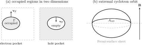
An electron pocket encloses occupied states and has outward electron velocity; a hole pocket encloses missing states and has inward electron velocity. Quantum oscillations measure an extremal cross-sectional area $A_{\mathrm{ext}}$ perpendicular to the magnetic field $\mathbf B$.

A hole is not a second microscopic particle hidden in the band. It is the convenient positive-charge description of a missing electron in an almost full band. Holes owns that filled-reference reorganization and its crystal-momentum and current signs; this page retains pocket geometry and compensation. The sign of the local curvature motivates electron-like or hole-like dynamics, but measured Hall and thermoelectric signs in a multiband material also depend on mobilities, scattering anisotropy, and interband effects.

Compensated semimetals

Suppose small electron and hole pockets coexist. Relative to a reference with filled valence bands and empty conduction bands, the carrier imbalance per primitive cell is

$$\delta\nu = \frac{\Omega_c}{(2\pi)^d} \left( \sum_a g_{e,a}V_{e,a} - \sum_b g_{h,b}V_{h,b} \right),$$

where $g_{e,a}$ and $g_{h,b}$ count degeneracies omitted from the pocket labels. A compensated semimetal satisfies

$$\sum_a g_{e,a}V_{e,a} = \sum_b g_{h,b}V_{h,b}.$$

Compensation is a state-counting statement. It does not imply zero conductivity, zero magnetoresistance, or a vanishing Hall coefficient.

Fermi-Surface Topology

The geometry of a Fermi surface includes more than its volume. Important data include:

• the number of connected sheets;
• whether a sheet is contractible or wraps around the Brillouin torus;
• the genus and neck structure of a three-dimensional sheet;
• symmetry-related copies and protected degeneracies;
• electron-like and hole-like orientation;
• proximity to band critical points;
• nesting vectors that connect extended, nearly parallel regions.

A Lifshitz transition occurs when a continuous change of chemical potential, pressure, strain, or another control parameter changes the topology of the Fermi surface. At the transition,

$$\varepsilon_n(\mathbf k_c) = \mu, \qquad \nabla_{\mathbf k} \varepsilon_n(\mathbf k_c) = 0.$$

Common possibilities are:

1. creation or annihilation of a pocket at a band extremum;
2. opening or pinching off of a neck at a saddle point;
3. reconnection of sheets across an identified Brillouin-zone boundary.

No broken symmetry is required. The nonanalyticity comes from the band critical point crossing the chemical potential. Thermodynamic derivatives and transport coefficients can show anomalies, while the associated van Hove singularity depends on dimension and local curvature.

This use of topology concerns the ordinary topology of constant-energy manifolds. It is distinct from topological-band invariants such as Chern numbers and $\mathbb Z_2$ indices.

Worked Example: An Ellipsoidal Pocket

Consider

$$\varepsilon(\mathbf k) = E_c + \frac{\hbar^2 k_x^2}{2m_x} + \frac{\hbar^2 k_y^2}{2m_y} + \frac{\hbar^2 k_z^2}{2m_z},$$

with $m_i>0$ and $\Delta=\mu-E_c>0$. The principal semiaxes are

$$k_{\mathrm F,i} = \frac{\sqrt{2m_i\Delta}}{\hbar}.$$

The occupied pocket volume is

$$V_{\mathrm F} = \frac{4\pi}{3} k_{\mathrm F,x} k_{\mathrm F,y} k_{\mathrm F,z}.$$

The velocity components are

$$v_i = \frac{\hbar k_i}{m_i}.$$

Unless all three masses are equal, $\mathbf v$ is not parallel to $\mathbf k$. For a magnetic field along $z$, the largest cross section perpendicular to the field occurs at $k_z=0$:

$$A_{\mathrm{ext}} = \pi k_{\mathrm F,x} k_{\mathrm F,y}.$$

The associated cyclotron mass is

$$m_c = \frac{\hbar^2}{2\pi} \left. \frac{\partial A(E)}{\partial E} \right|_{E=\mu} = \sqrt{m_xm_y}.$$

Thus rotating the field maps combinations of the principal masses and semiaxes.

Worked Example: Square-Lattice Topology Change

For a nearest-neighbor square lattice,

$$\varepsilon(\mathbf k) = -2t \left[ \cos(k_xa) + \cos(k_ya) \right], \qquad t>0.$$

The band minimum $-4t$ lies at $\Gamma=(0,0)$ and the maximum $4t$ at $M=(\pi/a,\pi/a)$. The points

$$X=(\pi/a,0), \qquad Y=(0,\pi/a)$$

are saddles at zero energy.

For $-4t<\mu<0$, the occupied region forms an electron-like sea around $\Gamma$. At half filling,

$$\mu=0, \qquad \cos(k_xa)+\cos(k_ya)=0,$$

and the Fermi contour passes through $X$ and $Y$. The Fermi velocity vanishes at those saddle points, the two-dimensional density of states diverges logarithmically in the ideal model, and the contour is at a Lifshitz transition.

For $0<\mu<4t$, it is more economical to describe the small unoccupied region around $M$ as a hole pocket. The occupied fraction changes continuously through $\mu=0$, but the contour topology and low-energy phase space do not.

Semiclassical Orbits in a Magnetic Field

Semiclassical Dynamics of Bloch Electrons owns the one-band equations and their weak-field validity tests. This section retains the constant-energy level-set geometry, open-versus-closed orbit classification, and inputs used by quantum-oscillation analysis.

For an electron of charge $-e$, with $e>0$, the owner’s uniform-field equation reduces to

$$\hbar\dot{\mathbf k} = -e\, \mathbf v_n(\mathbf k) \times \mathbf B.$$

On a continuous repeated-zone lift $\widetilde{\mathbf k}(t)$, the band energy and $\widetilde{\mathbf k}\cdot\mathbf B$ are conserved. The lifted orbit is therefore the intersection of a periodically continued constant-energy surface with a plane perpendicular to $\mathbf B$, and the physical path is its projection to the Brillouin torus. Closed projected orbits can be quantized; open orbits lead to qualitatively different magnetotransport and do not obey the simplest closed-orbit formulas.

Quantum Oscillations

Landau quantization causes successive cyclotron orbits to pass through the chemical potential as $B$ changes. The magnetization then oscillates in the de Haas–van Alphen effect, while transport coefficients oscillate in the Shubnikov–de Haas effect.

Quantum Oscillations owns the experimental workflow: field acquisition, background removal, inverse-field transforms, Lifshitz–Kosevich fits, reconstruction evidence, and phase cautions. This section supplies the orbit geometry and leading frequency dictionary used there.

For a closed orbit with cross-sectional area $A(E,k_\parallel)$ perpendicular to $\mathbf B$, semiclassical quantization has the form

$$A(E,k_\parallel) = \frac{2\pi eB}{\hbar} \left( j+\gamma \right),$$

where $\gamma$ contains the usual turning-point contribution and can be modified by Berry phase, orbital moment, and other corrections. The leading oscillation frequency is the Onsager relation

$$F = \frac{\hbar}{2\pi e} A_{\mathrm{ext}}.$$

$F$ is measured in tesla, and the signal is periodic in $1/B$:

$$\Delta \left( \frac{1}{B} \right) = \frac{1}{F}.$$

In three dimensions, contributions from neighboring planes generally dephase. Stationary-phase selection leaves extremal cross sections satisfying

$$\left. \frac{\partial A} {\partial k_\parallel} \right|_{\mathrm{ext}} = 0.$$

A single field orientation therefore reveals extremal areas, not the entire three-dimensional surface. Rotating the field and tracking frequencies performs a form of Fermi-surface tomography.

Cyclotron mass

The temperature dependence of an oscillation amplitude measures the orbit’s cyclotron mass,

$$m_c = \frac{\hbar^2}{2\pi} \left. \frac{\partial A(E)} {\partial E} \right|_{E=\mu}.$$

For the fundamental harmonic, the Lifshitz–Kosevich thermal factor is

$$R_T = \frac{X}{\sinh X}, \qquad X = \frac{2\pi^2k_{\mathrm B}T m_c} {\hbar eB}.$$

Elastic scattering produces a Dingle factor commonly written

$$R_D = \exp \left( -\frac{\pi} {\omega_c\tau_q} \right), \qquad \omega_c = \frac{eB}{m_c},$$

where $\tau_q$ is a quantum lifetime sensitive to Landau-level broadening. Transport and quantum lifetimes need not agree because they weight scattering angles differently.

Spin splitting, magnetic breakdown between nearby orbits, warping, chemical-potential oscillations, and interaction effects can all modify amplitudes and phases. A fitted phase offset is therefore not, by itself, a secure Berry-phase measurement.

Two-dimensional pocket count

For a two-dimensional pocket of area $A_{\mathrm F}$ and omitted degeneracy $g$,

$$n_{2\mathrm D} = g \frac{A_{\mathrm F}}{(2\pi)^2}.$$

Combining this with the Onsager relation gives

$$n_{2\mathrm D} = g \frac{eF}{h}.$$

The formula counts carriers per physical area for an isolated two-dimensional pocket. In a multiband material, each observed frequency must be assigned to an orbit before frequencies can be converted into a total carrier density.

What Experiments Actually Measure

No single experiment returns an assumption-free picture of the Fermi surface.

Probe	Primary information	Main cautions
ARPES	Occupied spectral function $A(\mathbf k,\omega)f(\omega)$ and band crossings	Surface sensitivity, matrix elements, finite resolution, and imperfect $k_z$ definition
Quantum oscillations	Extremal closed-orbit areas, cyclotron masses, and quantum lifetimes	Requires coherent high-mobility orbits; missing frequency does not prove a missing sheet
Hall and magnetotransport	Velocity-, curvature-, and lifetime-weighted carrier response	Multiband signs and densities are model dependent
STM/STS	Local density of states and, through interference, selected scattering vectors	Not a direct momentum-resolved occupation map
Compton scattering and positron annihilation	Bulk momentum-density information	Reconstruction is indirect and resolution limited

ARPES

In the sudden-approximation language, a photoemission intensity is schematically

$$I(\mathbf k,\omega) \propto |M(\mathbf k,\omega)|^2 f(\omega) A(\mathbf k,\omega),$$

convolved with instrumental resolution and broadened by backgrounds. A Fermi-level intensity map can trace band crossings, but dark matrix elements can hide real states and a broad incoherent spectrum may not define a sharp contour.

ARPES is momentum resolved and especially direct for quasi-two-dimensional materials. It is also surface sensitive, and the out-of-plane momentum inferred from photon energy relies on a final-state model. The Spectral Functions page explains what $A(\mathbf k,\omega)$ means beyond a noninteracting band picture.

Angle-Resolved Photoemission Spectroscopy owns the complete experimental treatment, including analyzer coordinates, energy and momentum resolution, $k_z$ scans, surface terminations, polarization selection, self-energy fits, and reproducibility.

Quantum oscillations

Quantum oscillations are bulk sensitive and extraordinarily precise for coherent closed pockets. They may nevertheless omit:

• sheets with masses too large for the available temperature and field;
• states with short quantum lifetime;
• open orbits;
• frequencies suppressed by spin zeros or magnetic breakdown;
• pockets outside the accessible field-orientation range.

Agreement between ARPES, quantum oscillations, thermodynamics, and band calculations is much stronger evidence than any one probe alone.

Hall sign is not a pocket census

In the weak-field two-carrier Drude model,

$$R_H = \frac{ n_h\mu_h^2-n_e\mu_e^2 }{ e \left( n_h\mu_h+n_e\mu_e \right)^2 },$$

where $\mu_e$ and $\mu_h$ are positive mobilities. Even at perfect compensation, $n_e=n_h$, the Hall coefficient vanishes only if the mobilities are equal. Anisotropic bands and scattering make the relation still less direct.

Drude Theory derives this weak-field result from the full conductivity tensor and shows why Hall sign is mobility weighted rather than a direct pocket census.

Interactions and Reconstruction

In a Fermi liquid, interactions renormalize the dispersion, velocity, residue, lifetime, and sometimes the apparent shape of the surface. A quasiparticle Fermi surface can be located by a zero of the real part of the inverse retarded Green function at zero energy,

$$\operatorname{Re} G^{-1}(\mathbf k,0) = 0,$$

provided a coherent low-energy pole exists. The occupation need not jump by one; its discontinuity is the quasiparticle residue $Z<1$.

Luttinger’s theorem constrains the total volume enclosed by the interacting Fermi surface for broad classes of translationally invariant fermion systems with conserved particle number and no relevant topological obstruction. Its application requires care:

• broken translational symmetry changes the primitive cell and folds the Brillouin zone;
• density waves hybridize folded bands and reconstruct large sheets into smaller pockets;
• spin polarization changes the spin-resolved volumes;
• topological order can modify the conventional volume relation;
• zeros of the Green function can matter in strongly correlated insulators and pseudogapped states.

In a superconductor, the ordinary electron Fermi surface is replaced by Bogoliubov excitations that are usually gapped except at nodes. Researchers may discuss an underlying normal-state Fermi surface, but that object is inferred from a model or from measurements above the transition. In a Mott insulator or a non-Fermi liquid with no sharp quasiparticle crossing, drawing a band-like Fermi surface can be misleading.

The Fermi-Liquid Theory Preview develops the interacting low-energy picture without duplicating the material-specific geometry here.

Why Low-Energy Metal Physics Lives Here

Pauli exclusion blocks most low-energy rearrangements deep inside the occupied sea. For a process with energy scale

$$E_* \sim \max \left( k_{\mathrm B}T,\hbar\omega \right),$$

only states in a shell of local thickness

$$\delta k_\perp \sim \frac{E_*} {\hbar|\mathbf v_{\mathrm F}|}$$

can readily change occupation. The enormous filled sea supplies the ground-state density, but the thin shell around its boundary supplies most low-temperature entropy, heat capacity, transport, and weak-coupling scattering phase space.

This logic explains several standard results:

• the electronic heat capacity is linear in $T$ when the density of states is regular;
• conductivity is a Fermi-surface integral weighted by velocities and lifetimes;
• screening and response functions are sensitive to vectors connecting points on the surface;
• pairing acts on states in an energy shell around the surface;
• nesting can enhance selected particle-hole responses;
• small velocities or van Hove proximity can amplify interaction effects.

The slogan needs two qualifications. First, filled bands can carry geometric and topological response even without a Fermi surface. Second, in incoherent or strongly correlated metals the relevant low-energy spectral weight may not be organized by long-lived quasiparticle sheets.

Patch description

Divide a smooth surface into patches labeled by $a$. Within one patch,

$$\xi_a(\mathbf q) \simeq \hbar v_{\mathrm F,a}q_\perp.$$

The tangential coordinates label many low-energy channels while only $q_\perp$ controls the leading excitation energy. A low-energy integral therefore has the schematic form

$$\int \frac{d^dk}{(2\pi)^d} \simeq \sum_a \int_{\mathrm{patch}\ a} \frac{dS_{\mathbf k}} {(2\pi)^d} \int dq_\perp.$$

This decomposition underlies Landau Fermi-liquid theory, patch renormalization groups, and many treatments of superconducting and density-wave instabilities.

Practical Workflow for a Calculated Band Structure

Band Structure Workflows owns the converged crystal calculation, electron count, full-zone bands, and artifact provenance supplied to this analysis. This page owns the chemical-potential level set, pocket geometry, volume checks, and probe-aware Fermi-surface interpretation.

To analyze a proposed Fermi surface:

1. State the primitive cell, reciprocal basis, Brillouin-zone convention, and whether spin is included in the band index.
2. Fix the electron count and determine $\mu$ using a converged Brillouin-zone integration.
3. Locate every band crossing $\mu$; do not infer a three-dimensional sheet from one high-symmetry path.
4. Build constant-energy contours or isosurfaces on a dense mesh and sew opposite zone faces.
5. Label connected sheets, degeneracies, electron or hole orientation, velocities, and symmetry copies.
6. Check the occupied-volume sum against the target filling.
7. Search for nearby critical points and quantify sensitivity to $\mu$, strain, spin–orbit coupling, and numerical interpolation.
8. For comparison with oscillations, compute extremal cross sections as a function of field orientation and the associated $\partial A/\partial E$.
9. For comparison with ARPES, include matrix-element, surface, $k_z$, and spectral-linewidth limitations.

The volume check is a powerful debugging tool. A beautiful isosurface with the wrong degeneracy or chemical potential is still the wrong Fermi surface.

Common Mistakes

Calling the filled region the Fermi surface

The Fermi sea is occupied volume; the Fermi surface is its boundary.

Treating one scalar as the Fermi wavevector

One $k_{\mathrm F}$ is special to isotropic or highly symmetric cases. Generic crystalline sheets require a function or parametrization.

Assuming velocity is parallel to crystal momentum

$\mathbf v_{\mathrm F}$ follows $\nabla_{\mathbf k}\varepsilon$, not the radius vector from an arbitrarily chosen zone origin.

Forgetting identified zone faces

A contour that exits one side of the plotted Brillouin zone re-enters at the reciprocal-lattice-equivalent side.

Classifying pockets from plot position alone

Electron or hole character follows occupation and local dispersion, not whether a contour happens to surround $\Gamma$ in one representation.

Multiplying degeneracy twice

If spin–orbit-coupled bands already include spin, an extra factor of two corrupts both filling and pocket density.

Equating Hall sign with the only carrier type

Multiband Hall response is mobility weighted and can change sign without a change in the number of electron-like and hole-like sheets.

Treating every oscillation frequency as a distinct pocket

Harmonics, magnetic breakdown, warping, spin splitting, and symmetry-related orbits can generate several frequencies from one underlying sheet.

Reading a Berry phase from an intercept alone

Dimensionality, Zeeman coupling, orbital moment, indexing choices, and field-dependent chemical potential can shift the phase.

Using band language where no coherent crossing exists

Mott phases, pseudogaps, superconductors, and non-Fermi liquids require spectral and symmetry qualifications.

Exercises

Exercise 1: filling and full bands

A two-dimensional crystal has primitive-cell area $\Omega_c$. Two nondegenerate bands are completely filled, and a third band has occupied area $A_{\mathrm{occ}}$ in the Brillouin zone. Find the number of electrons per cell represented by these bands. How does the answer change if every displayed band is spin degenerate but spin is not included in the band label?

Solution

The Brillouin-zone area is

$$A_{\mathrm{BZ}} = \frac{(2\pi)^2}{\Omega_c}.$$

Each full nondegenerate band contributes one electron per cell, while the partial band contributes

$$\frac{A_{\mathrm{occ}}} {A_{\mathrm{BZ}}} = \frac{\Omega_c A_{\mathrm{occ}}} {(2\pi)^2}.$$

Therefore

$$\nu = 2 + \frac{\Omega_c A_{\mathrm{occ}}} {(2\pi)^2}.$$

If spin degeneracy is omitted from every displayed band, multiply the entire result by two:

$$\nu = 4 + 2 \frac{\Omega_c A_{\mathrm{occ}}} {(2\pi)^2}.$$

The factor is applied once, not separately to the area and again to the band count.

Exercise 2: normal direction

Show that the Fermi velocity of the ellipsoidal band is normal to the ellipsoidal Fermi surface, even though it is generally not parallel to $\mathbf k$.

Solution

Define the surface by

$$\Phi(\mathbf k) = \frac{k_x^2}{k_{\mathrm F,x}^2} + \frac{k_y^2}{k_{\mathrm F,y}^2} + \frac{k_z^2}{k_{\mathrm F,z}^2} - 1 = 0.$$

Its normal is proportional to

$$\nabla_{\mathbf k}\Phi = 2 \left( \frac{k_x}{k_{\mathrm F,x}^2}, \frac{k_y}{k_{\mathrm F,y}^2}, \frac{k_z}{k_{\mathrm F,z}^2} \right).$$

Since

$$k_{\mathrm F,i}^2 = \frac{2m_i\Delta}{\hbar^2},$$

this normal is proportional to

$$\left( \frac{k_x}{m_x}, \frac{k_y}{m_y}, \frac{k_z}{m_z} \right).$$

But

$$\mathbf v = \hbar \left( \frac{k_x}{m_x}, \frac{k_y}{m_y}, \frac{k_z}{m_z} \right).$$

Hence $\mathbf v$ is normal to the surface. It is parallel to $\mathbf k$ only when the relevant masses are equal or when $\mathbf k$ lies on a principal axis.

Exercise 3: square-lattice Lifshitz point

Verify that the points $X=(\pi/a,0)$ and $Y=(0,\pi/a)$ are critical points of the nearest-neighbor square-lattice band and classify their local curvature.

Solution

The derivatives are

$$\frac{\partial\varepsilon}{\partial k_x} = 2ta\sin(k_xa), \qquad \frac{\partial\varepsilon}{\partial k_y} = 2ta\sin(k_ya).$$

Both vanish at $X$ and $Y$. Near $X$, write

$$k_x = \frac{\pi}{a}+q_x, \qquad k_y = q_y.$$

Using

$$\cos(\pi+q_xa) \simeq -1+\frac{a^2q_x^2}{2}, \qquad \cos(q_ya) \simeq 1-\frac{a^2q_y^2}{2},$$

gives

$$\varepsilon \simeq -ta^2 \left( q_x^2-q_y^2 \right).$$

The curvatures have opposite signs, so $X$ is a saddle; $Y$ is equivalent by symmetry. When $\mu$ crosses zero, the Fermi contour passes through these saddles and changes from electron-like to hole-like topology.

Exercise 4: oscillation frequency and carrier density

A spin-degenerate two-dimensional circular pocket produces a quantum-oscillation frequency $F$. Find its area and carrier density per physical area.

Solution

The Onsager relation gives

$$A_{\mathrm F} = \frac{2\pi e}{\hbar} F.$$

For spin degeneracy $g=2$,

$$n_{2\mathrm D} = 2 \frac{A_{\mathrm F}}{(2\pi)^2}.$$

Substitution yields

$$n_{2\mathrm D} = 2 \frac{eF}{h}.$$

This result assumes one isolated pocket and that the observed frequency is its fundamental extremal orbit rather than a harmonic or breakdown orbit.

Exercise 5: cyclotron mass of an ellipsoid

For the ellipsoidal band and $\mathbf B\parallel\hat{\mathbf z}$, derive $m_c=\sqrt{m_xm_y}$.

Solution

At fixed energy offset $\Delta_E=E-E_c$, the extremal section at $k_z=0$ has semiaxes

$$k_x(E) = \frac{\sqrt{2m_x\Delta_E}}{\hbar}, \qquad k_y(E) = \frac{\sqrt{2m_y\Delta_E}}{\hbar}.$$

Therefore

$$\begin{aligned} A(E) &= \pi k_x(E)k_y(E) \\ &= \frac{2\pi\Delta_E}{\hbar^2} \sqrt{m_xm_y}. \end{aligned}$$

Using the definition,

$$\begin{aligned} m_c &= \frac{\hbar^2}{2\pi} \frac{\partial A}{\partial E} \\ &= \sqrt{m_xm_y}. \end{aligned}$$

The mass along the field does not enter this orbit’s cyclotron mass.

Exercise 6: compensation does not fix the Hall sign

Use the weak-field two-carrier formula to determine the Hall coefficient of a compensated semimetal with $n_e=n_h=n$. Under what condition does it vanish?

Solution

Set $n_e=n_h=n$:

$$\begin{aligned} R_H &= \frac{ n\mu_h^2-n\mu_e^2 }{ e n^2 \left( \mu_h+\mu_e \right)^2 } \\ &= \frac{ (\mu_h-\mu_e) (\mu_h+\mu_e) }{ e n \left( \mu_h+\mu_e \right)^2 } \\ &= \frac{ \mu_h-\mu_e }{ e n \left( \mu_h+\mu_e \right) }. \end{aligned}$$

It vanishes only when $\mu_h=\mu_e$. The sign is hole-like if $\mu_h>\mu_e$ and electron-like if $\mu_e>\mu_h$, despite exact carrier compensation.

Exercise 7: the low-energy shell

Estimate the fraction of occupied states that lie within energy $E_*$ of the Fermi energy for a three-dimensional isotropic parabolic band. Assume $E_*\ll E_{\mathrm F}$.

Solution

For

$$\varepsilon = \frac{\hbar^2k^2}{2m},$$

the Fermi velocity is

$$v_{\mathrm F} = \frac{\hbar k_{\mathrm F}}{m}.$$

The shell thickness is

$$\delta k \simeq \frac{E_*}{\hbar v_{\mathrm F}} = \frac{mE_*}{\hbar^2k_{\mathrm F}}.$$

The shell volume just inside the surface is approximately

$$\delta V_k \simeq 4\pi k_{\mathrm F}^2\delta k,$$

while the sea volume is

$$V_{\mathrm F} = \frac{4\pi}{3}k_{\mathrm F}^3.$$

Their ratio is

$$\frac{\delta V_k}{V_{\mathrm F}} \simeq 3 \frac{\delta k}{k_{\mathrm F}} = \frac{3}{2} \frac{E_*}{E_{\mathrm F}}.$$

Only a parametrically small fraction of the sea participates in low-energy rearrangements, even though that shell controls much of the low-temperature response.

Connections

• The chapter gateway routes a declared coherent dispersion and filling to this material-facing geometry or redirects incoherent spectra to many-body owners.
• Metals, Insulators, and Semiconductors explains when a Fermi surface implies metallic transport and how semimetal, localization, and interaction-driven exceptions are classified.
• Band Theory Overview explains how Bloch bands are defined, filled, and interpreted before their chemical-potential level sets are extracted.
• Fermi Surface in Many-Body and Quantum Statistical Mechanics develops the generic occupation boundary, free gas, thermal shell, and interacting definition.
• Density of States derives the constant-energy-surface measure and van Hove singularities.
• Tight-Binding Models supplies lattice dispersions whose constant-energy contours become Fermi surfaces.
• Brillouin Zones explains reduced-zone geometry and reciprocal-face identification.
• Sommerfeld Expansion turns smooth Fermi-surface data into low-temperature thermodynamics.
• Fermi-Liquid Theory Preview introduces interacting quasiparticle surfaces and their low-energy lifetime.
• Itinerant Magnetism shows how Fermi-surface phase space selects uniform or finite-wavevector magnetic response and how order reconstructs the surface.
• Charge and Spin Density Waves distinguishes useful nesting geometry from a demonstrated instability and develops density-wave reconstruction.
• RKKY Interaction shows how Kohn anomalies, caliper vectors, curvature, and orbital matrix elements become long-range exchange between local moments.
• Stoner Criterion gives the uniform scalar stability test obtained by transferring particles between spin-resolved Fermi seas.
• Effective Mass derives local curvature tensors and the orbit-area definition of cyclotron mass.
• Angle-Resolved Photoemission Spectroscopy turns occupied spectral weight into calibrated energy–momentum cuts and Fermi-level maps with explicit surface and matrix-element controls.
• Quantum Oscillations turns extremal areas and cyclotron masses into an auditable Shubnikov–de Haas and de Haas–van Alphen analysis.
• Drude Theory connects carrier pockets to dc, Hall, magnetotransport, and optical response under an explicit relaxation-time model.
• Boltzmann Transport turns Fermi-surface velocities, state-dependent scattering, and thermal windows into electrical and thermoelectric tensors.
• Hall Effect explains why pocket geometry, mobility weighting, and multiband compensation obstruct a naive carrier-count interpretation.
• Weyl and Dirac Semimetals connects pointlike bulk Fermi surfaces, doped pockets, open surface arcs, and bulk–surface Weyl orbits.

References

1. N. W. Ashcroft and N. D. Mermin, Solid State Physics (Holt, Rinehart and Winston, 1976), Chapters 2, 12, 13, and 14.
2. M. P. Marder, Condensed Matter Physics, 2nd ed. (Wiley, 2010), Chapters 6 and 7.
3. S. H. Simon, The Oxford Solid State Basics (Oxford University Press, 2013), Chapters 4–7.
4. L. Onsager, “Interpretation of the de Haas–van Alphen effect,” The London, Edinburgh, and Dublin Philosophical Magazine and Journal of Science 43, 1006–1008 (1952), doi:10.1080/14786440908521019.
5. I. M. Lifshitz and A. M. Kosevich, “Theory of Magnetic Susceptibility in Metals at Low Temperature,” Soviet Physics JETP 2, 636–645 (1956), JETP archive.
6. D. Shoenberg, Magnetic Oscillations in Metals (Cambridge University Press, 1984), doi:10.1017/CBO9780511897870.
7. I. M. Lifshitz, “Anomalies of Electron Characteristics of a Metal in the High Pressure Region,” Soviet Physics JETP 11, 1130–1135 (1960), JETP archive.
8. J. M. Luttinger, “Fermi Surface and Some Simple Equilibrium Properties of a System of Interacting Fermions,” Physical Review 119, 1153–1163 (1960), doi:10.1103/PhysRev.119.1153.
9. A. Damascelli, Z. Hussain, and Z.-X. Shen, “Angle-resolved photoemission studies of the cuprate superconductors,” Reviews of Modern Physics 75, 473–541 (2003), doi:10.1103/RevModPhys.75.473.
10. J. A. Sobota, Y. He, and Z.-X. Shen, “Angle-resolved photoemission studies of quantum materials,” Reviews of Modern Physics 93, 025006 (2021), doi:10.1103/RevModPhys.93.025006.