Drude Theory

Drude theory is the single-relaxation-time model of charge-current response. It assumes that a carrier’s mean drift momentum accelerates under an electric field and relaxes exponentially toward equilibrium:

$$\frac{d\mathbf p_d}{dt} = q\mathbf E - \frac{\mathbf p_d}{\tau}.$$

For an isotropic parabolic band, $\mathbf p_d=m^*\mathbf v_d$. The resulting dc conductivity is

$$\sigma_0 = \frac{nq^2\tau}{m^*}.$$

This formula looks classical, but its successful modern use is usually Drude–Sommerfeld: carrier density comes from Fermi statistics and band filling, $m^*$ from a band or quasiparticle dispersion, and $\tau$ from momentum-relaxing scattering near the Fermi surface. The model does not predict those inputs. It organizes them into a low-frequency response.

This page owns the scalar and tensor Drude equations, relaxation-time interpretation, dc and ac conductivity, Hall response, optical spectral weight, fitting workflow, and failure tests. Transport Coefficients Preview owns generic transport limits and hydrodynamic classification, Kubo Formula owns the exact linear-response construction, and Effective Mass owns curvature, conductivity, cyclotron, and optical mass distinctions.

Required background. Effective Mass supplies the response-specific mass distinctions used here without rederivation.

Helpful background. Fermi Surface supplies low-energy phase space, Metals, Insulators, and Semiconductors supplies carrier and filling classification, and Transport Coefficients Preview supplies the bulk, ballistic, hydrodynamic, and limit-order taxonomy.

The Minimal Model

Let $q$ be the signed carrier charge. Thus $q=-e$ for an electron and $q=+e$ for a hole. The microscopic carrier velocity can be large even in equilibrium, but opposite directions cancel. $\mathbf v_d$ denotes only the small nonequilibrium drift average.

For an isotropic band and zero magnetic field,

$$m^* \frac{d\mathbf v_d}{dt} = q\mathbf E(t) - \frac{m^*\mathbf v_d}{\tau}.$$

The relaxation term asserts:

• linear response in the drift velocity;
• local, memoryless damping;
• one momentum-relaxation time $\tau$;
• a fixed carrier density and effective mass;
• spatially uniform response;
• no distinction among directions, bands, or points on the Fermi surface.

Those are model assumptions, not definitions of a metal.

Time-domain solution

After transients from the remote past have decayed,

$$\mathbf v_d(t) = \frac{q}{m^*} \int_{-\infty}^{t} dt'\, e^{-(t-t')/\tau} \mathbf E(t').$$

The response kernel is causal: only earlier fields contribute.

If a constant field $\mathbf E_0$ is switched on at $t=0$ and the initial drift is zero,

$$\mathbf v_d(t) = \frac{q\tau}{m^*} \mathbf E_0 \left( 1-e^{-t/\tau} \right).$$

If the field is switched off after steady state is reached, the current decays as $e^{-t/\tau}$. This is the operational meaning of the model’s relaxation time.

What relaxes

$\tau$ is a transport momentum-relaxation time. It need not equal:

• the interval between all microscopic collisions;
• a single-particle quantum lifetime from spectral broadening;
• a phase-coherence time;
• an energy-relaxation time;
• a recombination time;
• an escape time from a finite device.

A collision that changes momentum only slightly can strongly broaden a single-particle phase while relaxing current inefficiently. Naming the lifetime is part of reporting it.

DC Conductivity

In a time-independent field, the steady drift is

$$\mathbf v_d = \frac{q\tau}{m^*} \mathbf E.$$

The current density is

$$\mathbf j = nq\mathbf v_d.$$

Although electron drift is opposite to $\mathbf E$, multiplying by the negative electron charge makes the conventional current parallel to $\mathbf E$. Therefore

$$\mathbf j = \sigma_0\mathbf E, \qquad \sigma_0 = \frac{nq^2\tau}{m^*}.$$

The resistivity is

$$\rho_0 = \frac{1}{\sigma_0} = \frac{m^*}{nq^2\tau}.$$

Define the positive mobility

$$\mu = \frac{|q|\tau}{m^*}.$$

Then

$$\sigma_0 = n|q|\mu.$$

Conductivity is a bulk coefficient. Conductance also depends on sample geometry and contacts. For a uniform bar of length $L$ and cross-sectional area $A$,

$$G = \sigma_0 \frac{A}{L},$$

only when current distribution and contact effects permit the elementary geometry reduction.

Classical Equation, Quantum Inputs

The original Drude model treated carriers as a classical gas. That picture gives incorrect electronic heat capacity and misses Pauli blocking, band structure, and Fermi-surface geometry. Modern use keeps the momentum-balance equation while replacing its inputs.

Carrier density

$n$ is obtained from the occupied electronic states, not from a classical Maxwell distribution. In a simple monovalent metal it may be comparable to one carrier per atom; in a doped semiconductor or semimetal it can be many orders of magnitude smaller. In a multiband system there is no single $n$ unless a reduction is justified.

Effective mass

$m^*$ is a band, optical, or quasiparticle response parameter. It can be anisotropic, density dependent, or renormalized by interactions. Inserting the bare electron mass merely because the charge carrier is an electron is generally unjustified.

Fermi velocity and mean free path

In a degenerate metal, the characteristic velocity for transport is the Fermi velocity rather than a classical thermal velocity. The transport mean free path is

$$\ell_{\mathrm{tr}} = v_{\mathrm F}\tau_{\mathrm{tr}}.$$

This connects a time-domain Drude parameter with a spatial semiclassical criterion.

Boltzmann reduction

Boltzmann Transport owns the distribution function, collision operator, scattering-in terms, thermoelectric moments, and conservation tests. Its simplest weak-field relaxation-time reduction gives

$$\begin{aligned} \sigma_{ij} = q^2 \sum_n \int \frac{d^dk}{(2\pi)^d} &\left( - \frac{\partial f} {\partial\varepsilon} \right) \\ &\times v_{n,i}(\mathbf k) v_{n,j}(\mathbf k) \tau_n(\mathbf k). \end{aligned}$$

Only states in the thermal window around the chemical potential contribute through $-\partial f/\partial\varepsilon$. For one isotropic parabolic band and constant $\tau$, the integral reduces to $nq^2\tau/m^*$.

For an isotropic degenerate band, the same physics can be written as an Einstein relation,

$$\sigma = q^2 \rho(E_{\mathrm F}) D,$$

with

$$D = \frac{v_{\mathrm F}^2\tau}{d}.$$

Here $\rho(E_{\mathrm F})$ is the density of states per volume, including the degeneracies used in $n$. The Drude and diffusion forms agree only when their masses, state counts, and scattering approximations describe the same carriers.

Tensor Drude Response

For a parabolic band with mass tensor $\mathsf M$ and scalar relaxation time,

$$\frac{d\mathbf v_d}{dt} + \frac{\mathbf v_d}{\tau} = q\mathsf M^{-1}\mathbf E.$$

The dc conductivity tensor is

$$\boldsymbol\sigma_0 = nq^2\tau \mathsf M^{-1}.$$

In principal axes,

$$\sigma_{ii} = \frac{nq^2\tau}{m_i}.$$

If $\tau$ is also anisotropic or momentum dependent, it cannot in general be represented by multiplying $\mathsf M^{-1}$ by one scalar. A measured conductivity anisotropy can come from mass, Fermi-surface geometry, scattering, carrier density, or all four.

Effective Mass distinguishes the tensor, conductivity, density-of-states, cyclotron, and optical masses used in such reductions.

AC Conductivity

Use the convention

$$\mathbf E(t) = \operatorname{Re} \left[ \mathbf E_\omega e^{-i\omega t} \right].$$

The drift equation gives

$$\mathbf v_\omega = \frac{q/m^*} {\tau^{-1}-i\omega} \mathbf E_\omega.$$

Therefore

$$\sigma(\omega) = \frac{nq^2/m^*} {\tau^{-1}-i\omega} = \frac{\sigma_0} {1-i\omega\tau}.$$

The pole lies at $\omega=-i/\tau$, in the lower half-plane as required for a retarded response.

The dissipative and reactive parts are

$$\operatorname{Re}\sigma(\omega) = \frac{\sigma_0} {1+\omega^2\tau^2},$$ $$\operatorname{Im}\sigma(\omega) = \frac{\sigma_0\omega\tau} {1+\omega^2\tau^2}.$$

The cycle-averaged absorbed power density is

$$\overline P = \frac{1}{2} \operatorname{Re}\sigma(\omega) |\mathbf E_\omega|^2.$$

$\operatorname{Re}\sigma$ is a Lorentzian centered at zero frequency with half width

$$\gamma = \frac{1}{\tau}.$$

For $\omega\tau\ll1$, the current nearly follows the field. For $\omega\tau\gg1$, collisions are too slow to establish the dc drift during one cycle and the response is mainly reactive:

$$\sigma(\omega) \approx i \frac{nq^2} {m^*\omega}.$$

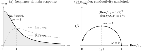
For $\sigma/\sigma_0=(1-i\omega\tau)^{-1}$, the dissipative peak has half width $1/\tau$, while the reactive part peaks at $\omega\tau=1$. At positive frequency the complex conductivity traces the upper semicircle from $\sigma/\sigma_0=1$ toward the origin.

Spectral Weight and the Clean Limit

Write

$$\mathcal D_0 = \frac{nq^2}{m^*}.$$

Then

$$\operatorname{Re}\sigma(\omega) = \mathcal D_0 \frac{\gamma} {\gamma^2+\omega^2}.$$

The positive-frequency intraband area is

$$\int_0^\infty d\omega\, \operatorname{Re}\sigma(\omega) = \frac{\pi}{2} \frac{nq^2}{m^*}.$$

Changing $\tau$ changes the width and height but not this Drude area. In the clean limit,

$$\lim_{\gamma\to0^+} \frac{\gamma} {\gamma^2+\omega^2} = \pi\delta(\omega)$$

on the full frequency axis. Thus

$$\operatorname{Re}\sigma(\omega) \longrightarrow \pi\mathcal D_0 \delta(\omega).$$

Different communities absorb factors of $\pi$ into the definition of “Drude weight.” A quoted Drude weight must include its conductivity convention.

In a continuum parabolic model, the full optical $f$-sum is governed by the bare mass. In a lattice, low-frequency intraband weight can involve band curvature and interactions, while interband transitions carry the remaining spectral weight. A partial Drude integral is not automatically the full sum rule.

Sum Rules owns exact integrated spectral constraints. The delta-function distinction between an ideal conductor and an insulator is broader than a finite-$\tau$ fit and connects to Metals, Insulators, and Semiconductors.

Dielectric Function and Plasma Scale

For the $e^{-i\omega t}$ convention,

$$\epsilon(\omega) = \epsilon_\infty + \frac{i\sigma(\omega)} {\epsilon_0\omega}.$$

Define the Drude plasma frequency

$$\omega_p^2 = \frac{nq^2} {\epsilon_0m^*}.$$

Then

$$\epsilon(\omega) = \epsilon_\infty - \frac{\omega_p^2} {\omega \left( \omega+i/\tau \right)}.$$

The zero of the longitudinal dielectric function controls a bulk plasma mode after background screening and damping are included. Reflectivity edges, loss-function peaks, and zeros of $\operatorname{Re}\epsilon$ need not coincide when absorption or interband structure is appreciable.

Plasmons Preview owns self-consistent charge oscillations, dimensional scaling, dielectric zeros, and damping.

Magnetic Field and the Hall Effect

Include a static magnetic field:

$$m^* \frac{d\mathbf v_d}{dt} = q \left( \mathbf E + \mathbf v_d\times\mathbf B \right) - \frac{m^*\mathbf v_d}{\tau}.$$

Take $\mathbf B=B\hat{\mathbf z}$ and define the signed cyclotron frequency and field parameter

$$\omega_c = \frac{qB}{m^*}, \qquad \beta_c = \omega_c\tau.$$

In steady state,

$$\boldsymbol\sigma = \frac{\sigma_0} {1+\beta_c^2} \begin{pmatrix} 1 & \beta_c \\ -\beta_c & 1 \end{pmatrix}.$$

The resistivity tensor is

$$\boldsymbol\rho = \frac{1}{\sigma_0} \begin{pmatrix} 1 & -\beta_c \\ \beta_c & 1 \end{pmatrix}.$$

With the convention

$$R_H = \frac{E_y} {j_xB} = \frac{\rho_{yx}}{B},$$

the single-carrier Hall coefficient is

$$R_H = \frac{1}{nq}.$$

It is negative for electrons and positive for holes. The Hall angle has magnitude

$$|\tan\theta_H| = |\omega_c\tau|.$$

The same one-band isotropic model predicts

$$\rho_{xx}(B) = \rho_0.$$

That is, it has zero transverse magnetoresistance despite a field-dependent $\sigma_{xx}$. Inverting the conductivity tensor matters. Observed magnetoresistance requires additional structure such as multiple carriers, anisotropy, momentum-dependent scattering, open orbits, inhomogeneity, or quantum effects.

Two-carrier response

For carrier species $a$ with positive mobility $\mu_a$ and sign $s_a=\operatorname{sgn}(q_a)$,

$$\sigma_{xx}(B) = \sum_a \frac{ n_a|q_a|\mu_a }{ 1+\mu_a^2B^2 },$$ $$\sigma_{xy}(B) = \sum_a \frac{ s_a n_a|q_a| \mu_a^2B }{ 1+\mu_a^2B^2 }.$$

For electrons of density $n$ and holes of density $p$, the weak-field Hall coefficient is

$$R_H = \frac{ p\mu_h^2 - n\mu_e^2 }{ e \left( p\mu_h+n\mu_e \right)^2 }.$$

The Hall sign is mobility weighted. A positive $R_H$ does not prove that every Fermi-surface sheet is hole-like, and $1/(eR_H)$ is not generally the total carrier density. Fermi Surface develops this warning in the context of electron and hole pockets.

What the Relaxation Time Contains

The Drude equation does not calculate $\tau$. Candidate momentum-relaxing mechanisms include:

• impurities, defects, and isotope disorder;
• phonons;
• electron–electron Umklapp;
• boundaries and interfaces;
• magnetic fluctuations;
• coupling to other collective modes;
• spatial inhomogeneity.

Transport versus quantum lifetime

For elastic scattering on an isotropic Fermi surface, a representative transport rate is

$$\frac{1}{\tau_{\mathrm{tr}}} = \sum_{\mathbf k'} W_{\mathbf k\mathbf k'} \left( 1-\cos\theta \right).$$

$\theta$ is the angle through which the velocity is scattered. The corresponding single-particle or quantum rate lacks the current-relaxation factor:

$$\frac{1}{\tau_q} = \sum_{\mathbf k'} W_{\mathbf k\mathbf k'}.$$

Forward scattering can make $\tau_{\mathrm{tr}}\gg\tau_q$. Comparing mobility and quantum-oscillation damping as though they measured one lifetime can therefore be misleading.

Matthiessen’s rule

Independent weak scattering channels are often approximated by

$$\frac{1}{\tau_{\mathrm{tr}}} \approx \sum_a \frac{1}{\tau_a}.$$

This is Matthiessen’s rule. It can fail when channels interfere, scattering is strongly energy dependent or anisotropic, the band structure changes with temperature, or one process modifies the distribution sampled by another.

A measured temperature dependence of $\rho$ is not predicted by Drude theory until a microscopic or empirical $\tau(T)$ is supplied.

Why Drude Works Surprisingly Often

The model survives because it is more general as a momentum-balance structure than its classical origin suggests.

One slow current-carrying mode

If the uniform current overlaps mainly with one slowly relaxing quantity, its low-frequency response often has one dominant pole:

$$\sigma(\omega) \sim \frac{\mathcal D} {\Gamma-i\omega}.$$

Microscopic quantum mechanics determines the weight $\mathcal D$ and relaxation rate $\Gamma$. The line shape can look Drude-like even when carriers are Bloch quasiparticles rather than classical balls between collisions.

Fermi statistics repair the thermodynamics

Only states near the Fermi surface respond to a weak field. This removes the classical prediction that every conduction electron contributes a thermal kinetic energy of order $k_{\mathrm B}T$ while preserving the simple conductivity reduction in a parabolic band.

Conservation laws protect momentum

Many collisions rapidly establish local equilibrium while relaxing total momentum only weakly. Uniform conductivity is then governed by the slower momentum-relaxing processes. A single long $\tau$ can summarize this bottleneck over a limited frequency range.

Low-frequency fitting can be forgiving

If experimental frequencies satisfy $\omega\tau\ll1$, many details collapse into the measured ratio $n\tau/m^*$. Good agreement with $\rho_0$ alone therefore validates that combination, not each microscopic parameter separately.

Wiedemann–Franz consistency

For a degenerate Fermi gas with sufficiently elastic, weakly energy-dependent scattering,

$$\frac{\kappa_e} {\sigma T} \longrightarrow L_0, \qquad L_0 = \frac{\pi^2}{3} \left( \frac{k_{\mathrm B}}{e} \right)^2.$$

The quantum Sommerfeld calculation supplies the correct Lorenz number. Deviations can arise from inelastic scattering, additional heat carriers, multiband structure, hydrodynamics, or non-Fermi-liquid behavior.

Extended Drude and Memory Diagnostics

A general causal intraband response can be parameterized as

$$\sigma(\omega) = \frac{\epsilon_0\omega_p^2} {M(\omega)-i\omega},$$

where $M(\omega)$ is a memory function. Ordinary Drude theory takes

$$M(\omega) = \frac{1}{\tau}.$$

Given a chosen intraband plasma frequency, optical analyses sometimes define

$$\frac{1} {\tau_{\mathrm{op}}(\omega)} = \epsilon_0\omega_p^2 \operatorname{Re} \left[ \frac{1}{\sigma(\omega)} \right],$$ $$\frac{m_{\mathrm{op}}(\omega)} {m_b} = - \frac{\epsilon_0\omega_p^2} {\omega} \operatorname{Im} \left[ \frac{1}{\sigma(\omega)} \right].$$

For a perfect Drude response these give $1/\tau$ and $1$. For real data they are derived optical functions, not direct measurements of a microscopic collision clock and mass. Their values depend on the chosen plasma frequency and on how interband, phonon, and collective contributions are subtracted.

Where Drude Fails

The model is unreliable when its one-fluid, local, memoryless assumptions fail.

Multiple bands or carrier types

Different densities, masses, charges, and lifetimes produce several response scales. One Drude peak can fit a limited interval while assigning physically false $n$, $m^*$, and $\tau$.

Nonparabolic or anisotropic bands

Current is a Fermi-surface average of velocities and scattering. A scalar mass cannot represent strongly warped surfaces, open orbits, or momentum-dependent $\tau$.

Interband and collective absorption

Optical conductivity can contain interband transitions, phonons, excitons, plasmons, density-wave modes, and superconducting condensate weight. Fitting all low-energy structure with one broadened Drude term violates spectral accounting.

Localization and hopping

Localized carriers do not support the same extended semiclassical drift. Activated hopping, variable-range hopping, weak localization, and Anderson localization require different frequency and temperature dependence.

Bad-metal and incoherent regimes

When

$$k_{\mathrm F}\ell_{\mathrm{tr}} \lesssim 1,$$

the picture of well-defined momentum between separated collisions becomes suspect. This Mott–Ioffe–Regel criterion is a heuristic crossover, not a universal sharp bound. Some correlated systems have broad, non-Drude conductivity without long-lived electron quasiparticles.

Hydrodynamic transport

Momentum-conserving electron–electron collisions can be much faster than momentum relaxation. The system can form a viscous electron fluid whose geometry-dependent flow is not captured by one local $\tau$.

Ballistic and mesoscopic transport

When device dimensions are shorter than the relevant mean free path, leads, channels, contacts, and transmission probabilities control conductance. A bulk Drude resistivity is no longer the complete protocol.

Strong magnetic field

When Landau quantization, quantum oscillations, magnetic breakdown, or edge states matter, the smooth classical Lorentz-force solution is incomplete.

Anomalous and topological Hall effects

Berry curvature, skew scattering, side jump, magnetic texture, and quantized Hall response generate transverse currents not reducible to $R_H=1/(nq)$.

Superconductivity

A superconductor transfers spectral weight into a zero-frequency condensate response and develops gap-dependent absorption. A narrow normal Drude peak alone cannot represent phase stiffness or the superconducting state.

Nonlinear and nonlocal response

Large fields can heat or redistribute carriers, while short wavelengths and anomalous skin effects make $\mathbf j(\mathbf r)$ depend on fields elsewhere. The local linear relation $\mathbf j=\sigma\mathbf E$ then needs replacement.

Using Drude Fits Responsibly

DC data

From $\rho_0$ alone one obtains only

$$\frac{n\tau}{m^*} = \frac{1} {q^2\rho_0}.$$

Separating $n$, $m^*$, and $\tau$ requires independent information. Hall density is independent only in a validated one-carrier regime. Optical weight, quantum oscillations, ARPES, capacitance, chemistry, and band calculations each bring their own assumptions.

Hall data

Measure both longitudinal and transverse voltages, antisymmetrize the Hall signal in $B$, symmetrize the longitudinal signal, and invert the full resistivity tensor when fitting conductivity components. Nonlinearity in $\rho_{yx}(B)$ is evidence against the weakest one-carrier reduction, but a linear curve alone does not prove it.

Optical data

Fit complex $\sigma(\omega)$ or an electrodynamically consistent reflectivity/transmission model, not only one visible peak. State:

• the Fourier convention;
• frequency range and resolution;
• background dielectric constant;
• interband and phonon components;
• number of Drude terms;
• fitted plasma frequencies and scattering rates;
• partial-sum cutoff;
• Kramers–Kronig or causal-model procedure.

Optics measures Drude weight and width. It does not separately determine $n$ and $m^*$ without another constraint.

Cross-probe ledger

Observable	Simple Drude inference	Required warning
$\rho_0$	$m^*/(nq^2\tau)$	only one parameter combination
weak-field $R_H$	$1/(nq)$	one isotropic carrier
mobility $\mu$	$	q
optical width	$1/\tau$	transport and optical lifetime may differ
Drude area	$\pi nq^2/(2m^*)$	partial weight and background subtraction
magnetoresistance	zero	nonzero response signals physics beyond scalar one-band Drude

A trustworthy interpretation seeks one set of carriers and conventions that explains several observables, while allowing response-specific masses and lifetimes where theory requires them.

Common Mistakes

• Using the bare electron mass without checking the band or optical mass.
• Calling every collision time a transport relaxation time.
• Inferring $n=1/(eR_H)$ in a multiband or anomalous-Hall material.
• Forgetting to invert the conductivity or resistivity tensor in a magnetic field.
• Fitting only $\operatorname{Re}\sigma$ without a causal complex response.
• Treating a numerical broadening as $1/\tau$.
• Adding scattering rates by Matthiessen’s rule without testing independence.
• Using a classical thermal velocity instead of $v_{\mathrm F}$ for a degenerate metal.
• Reading a successful dc fit as proof of coherent quasiparticles.
• Calling a zero-frequency delta function a finite resistivity.
• Ignoring interband spectral weight when applying an optical sum.
• Reporting a mobility, plasma frequency, or Hall density without units, geometry, temperature, field, and model.

Exercises

1. Current after a field step

A uniform field $\mathbf E_0$ is switched on at $t=0$. If $\mathbf j(0)=0$, derive $\mathbf j(t)$.

Solution

The current obeys

$$\frac{d\mathbf j}{dt} + \frac{\mathbf j}{\tau} = \frac{nq^2}{m^*} \mathbf E_0.$$

The solution is

$$\mathbf j(t) = \sigma_0\mathbf E_0 \left( 1-e^{-t/\tau} \right),$$

where

$$\sigma_0 = \frac{nq^2\tau}{m^*}.$$

At short times the current grows approximately linearly; at long times it reaches the dc value.

2. Drude spectral weight

Verify the positive-frequency area of the dissipative conductivity.

Solution

Using

$$\operatorname{Re}\sigma(\omega) = \frac{\sigma_0} {1+\omega^2\tau^2},$$

set $x=\omega\tau$:

$$\begin{aligned} \int_0^\infty d\omega\, \operatorname{Re}\sigma &= \frac{\sigma_0}{\tau} \int_0^\infty \frac{dx}{1+x^2} \\ &= \frac{\sigma_0}{\tau} \frac{\pi}{2} \\ &= \frac{\pi}{2} \frac{nq^2}{m^*}. \end{aligned}$$

The area is independent of $\tau$.

3. An illustrative metal

Take

$$n = 5.0\times10^{28}\,\mathrm{m^{-3}}, \qquad \rho_0 = 2.0\times10^{-8}\,\Omega\,\mathrm m,$$

with $m^*=m_e$ and $v_{\mathrm F}=1.5\times10^6\,\mathrm{m\,s^{-1}}$. Estimate $\tau$, mobility, and mean free path.

Solution

From $\rho_0=m_e/(ne^2\tau)$,

$$\tau = \frac{m_e} {ne^2\rho_0} \approx 3.6\times10^{-14}\,\mathrm s.$$

The mobility is

$$\mu = \frac{e\tau}{m_e} \approx 6.3\times10^{-3}\, \mathrm{m^2\,V^{-1}\,s^{-1}},$$

or about $63\,\mathrm{cm^2\,V^{-1}\,s^{-1}}$. The mean free path is

$$\ell = v_{\mathrm F}\tau \approx 5.4\times10^{-8}\,\mathrm m,$$

about $54\,\mathrm{nm}$. These values inherit the assumed one-band mass and density.

4. Hall coefficient and magnetoresistance

For one electron-like carrier, determine the Hall coefficient and longitudinal resistivity in a magnetic field.

Solution

With $q=-e$,

$$R_H = \frac{1}{nq} = -\frac{1}{ne}.$$

The inverse of the one-band conductivity tensor gives

$$\rho_{xx}(B) = \frac{1}{\sigma_0} = \frac{m^*}{ne^2\tau},$$

independent of $B$. Thus the isotropic one-carrier Drude model has a negative Hall coefficient and zero transverse magnetoresistance.

5. Mobility-weighted Hall sign

A compensated semimetal has $n=p$, but $\mu_h=2\mu_e$. What is the sign of its weak-field Hall coefficient?

Solution

For $n=p$,

$$R_H = \frac{ n\mu_h^2-n\mu_e^2 }{ en^2 \left( \mu_h+\mu_e \right)^2 }.$$

Since

$$\mu_h^2-\mu_e^2 = 4\mu_e^2-\mu_e^2 > 0,$$

$R_H$ is positive. The material is exactly carrier compensated, yet the more mobile holes control the weak-field Hall sign.

6. Forward scattering

Suppose scattering is concentrated at a small angle $\theta_0\ll1$. Compare its contributions to $1/\tau_q$ and $1/\tau_{\mathrm{tr}}$.

Solution

The quantum rate counts the event with weight approximately one. The transport rate includes

$$1-\cos\theta_0 \approx \frac{\theta_0^2}{2}.$$

Thus the same forward-scattering channel contributes much less to current relaxation:

$$\frac{ \tau_{\mathrm{tr}}^{-1} }{ \tau_q^{-1} } \sim \frac{\theta_0^2}{2}.$$

Consequently $\tau_{\mathrm{tr}}$ can be much longer than $\tau_q$.

7. Diagnose a non-Drude spectrum

An optical conductivity has a narrow zero-frequency peak, a broad mid-infrared band, and a frequency-dependent $1/\tau_{\mathrm{op}}(\omega)$. Is a single Drude fit a complete interpretation?

Solution

No. A defensible analysis should:

1. fit the full complex response over a declared range;
2. test whether more than one intraband component is required;
3. identify possible interband, phonon, collective, or localization contributions to the mid-infrared band;
4. check spectral-weight transfer as temperature or tuning changes;
5. state the plasma frequency used to define the extended-Drude functions;
6. compare dc conductivity with the $\omega\to0$ limit;
7. test Kramers–Kronig consistency and resolution effects;
8. compare carrier densities and masses with Hall, quantum-oscillation, photoemission, or band information.

The narrow component may be Drude-like, but the broad band and frequency-dependent memory show that one constant $\tau$ does not describe the entire spectrum.

Connections

• Terahertz and Infrared Probes develops the field- and power-resolved experimental workflow that turns a sample stack into complex optical conductivity and tests a Drude fit.
• Transport Measurements shows how terminal records, contact configurations, geometry, reversal, and tensor inversion produce the experimental conductivity to which a Drude model may be fitted.
• Boltzmann Transport resolves state-dependent velocities, collision integrals, electric and thermal driving, and the limits of a diagonal relaxation time.
• Disorder in Quantum Matter defines disorder ensembles and distinguishes the transport time controlling the Drude width from quantum and single-particle lifetimes.
• Weak Localization adds the leading phase-coherent interference correction to this classical diffusive baseline and fixes its magnetoconductance sign convention.
• Anderson Insulators replaces the extended-state Drude picture by localized orbitals, bath-assisted hopping, and Coulomb-gap transport.
• Hall Effect develops sign conventions, multiband tensor inversion, anomalous mechanisms, experimental extraction, and the bridge to quantization.
• Transport Coefficients Preview develops diffusion, Einstein relations, ballistic and hydrodynamic regimes, Green–Kubo formulas, and orders of limits.
• Kubo Formula derives conductivity from equilibrium current response and keeps electromagnetic contact terms explicit.
• Density Operators and Current Operators constructs microscopic currents and continuity equations.
• Lifetime and Spectral Weight distinguishes transport, quantum, coherence, and decay times.
• Fermi Surface connects carrier pockets, velocities, quantum oscillations, and multiband Hall warnings.
• Effective Mass explains which response-specific mass belongs in a Drude reduction.
• Fermi Liquid Theory Preview treats quasiparticle renormalization, backflow, and conservation constraints.
• Strange Metals audits when a measured linear resistivity can be converted into a Planckian rate and why that conversion is model dependent.
• Kondo Effect provides a concrete failure of a temperature-independent lifetime through many-body spin-flip scattering and strong-coupling saturation.
• Quantum Matter Conventions fixes Fourier signs, charge signs, tensor order, and conductivity normalization.
• Condensed Matter Roadmap places Drude theory between band structure and more general Boltzmann, Kubo, and mesoscopic transport.

References

• P. Drude, “Zur Elektronentheorie der Metalle,” Annalen der Physik 306, 566–613 (1900), doi:10.1002/andp.19003060312.
• A. Sommerfeld, “Zur Elektronentheorie der Metalle auf Grund der Fermischen Statistik. I,” Zeitschrift für Physik 47, 1–32 (1928), doi:10.1007/BF01391052.
• N. W. Ashcroft and N. D. Mermin, Solid State Physics, Holt, Rinehart and Winston, 1976.
• J. M. Ziman, Electrons and Phonons: The Theory of Transport Phenomena in Solids, Oxford University Press, 1960; Oxford Classic Texts reissue, 2001, doi:10.1093/acprof:oso/9780198507796.001.0001.
• M. Dressel and G. Grüner, Electrodynamics of Solids, Cambridge University Press, 2002, doi:10.1017/CBO9780511606168.
• R. Kubo, “Statistical-Mechanical Theory of Irreversible Processes. I,” Journal of the Physical Society of Japan 12, 570–586 (1957), doi:10.1143/JPSJ.12.570.
• W. Kohn, “Theory of the Insulating State,” Physical Review 133, A171–A181 (1964), doi:10.1103/PhysRev.133.A171.
• N. D. Mermin, “Lindhard Dielectric Function in the Relaxation-Time Approximation,” Physical Review B 1, 2362–2363 (1970), doi:10.1103/PhysRevB.1.2362.
• D. N. Basov, R. D. Averitt, D. van der Marel, M. Dressel, and K. Haule, “Electrodynamics of Correlated Electron Materials,” Reviews of Modern Physics 83, 471–541 (2011), doi:10.1103/RevModPhys.83.471.