Fermi Liquid Theory Preview

A Landau Fermi liquid is an interacting fermionic phase whose sufficiently low-energy excitations are long-lived quasiparticles labeled by points near a Fermi surface. The quasiparticles have renormalized energies and interact through a forward-scattering function, yet become asymptotically sharper as their excitation energy and temperature approach zero.

This is a low-energy statement, not a claim that the microscopic interaction is weak. Liquid helium-3, dilute atomic Fermi gases on their normal side, nuclear matter in suitable regimes, and many ordinary metals can all display Fermi-liquid behavior even though their microscopic Hamiltonians look very different.

The central organizing idea is economical:

$$\begin{gathered} \text{interacting many-fermion system} \\ \Downarrow \\ \text{Fermi surface} \\ \;+\; \text{long-lived quasiparticles} \\ \;+\; \text{residual forward interactions}. \end{gathered}$$

That change of variables predicts thermodynamics, static response, collisionless collective motion, and the scaling of decay rates. It also supplies precise failure tests. A system may possess a Fermi surface without possessing Landau quasiparticles.

Scope and Canonical Ownership

This page owns the generic Landau framework:

• adiabatic continuity and its limitations;
• the quasiparticle pole near a Fermi surface;
• the Landau energy functional;
• spin-symmetric and spin-antisymmetric Landau parameters;
• effective-mass and thermodynamic-response relations;
• Pomeranchuk stability conditions;
• the Landau kinetic equation and the simplest zero-sound condition;
• the low-energy lifetime law and its dimensional qualifications;
• practical diagnostics for conventional Fermi-liquid behavior.

Several neighboring pages remain canonical for details:

• Fermi Surface owns Fermi-sea geometry, state counting, Fermi velocity, and volume relations.
• Quasiparticles Overview owns the general particle-like criteria, dressing mechanisms, and quasiparticle taxonomy.
• Particle–Hole Excitations owns continuum kinematics and hole conventions.
• Spectral Functions owns residue normalization, linewidth conventions, and the distinction between intrinsic and displayed broadening.
• Lifetime and Spectral Weight owns the cross-system width, residue, propagation, and lifetime-convention audit; this page owns the Fermi-liquid scaling law.
• Susceptibilities owns source, detector, units, and order-of-limits conventions.
• Transport Coefficients Preview owns conductivity, diffusion, viscosity, Drude weight, and transport-limit definitions.
• Collective Modes owns the general response-pole and mode-classification language.
• Effective Mass owns the band-curvature formula card.

The discussion below is deliberately explicit about assumptions. Most compact formulas use a homogeneous, isotropic, parity-invariant, spin-rotation-invariant, three-dimensional normal Fermi liquid with one spherical Fermi surface. Lattice, multiband, anisotropic, two-dimensional, and spin-orbit-coupled systems require generalizations.

Convention Ledger

Momentum and state sums

The symbol $\mathbf p$ denotes physical momentum, so

$$\mathbf p = \hbar\mathbf k.$$

For a box of volume $\mathcal V$,

$$\frac1{\mathcal V} \sum_{\mathbf p} \longrightarrow \int \frac{d^3p} {(2\pi\hbar)^3}.$$

The spin label is

$$\sigma = \pm1$$

for the two components of a spin-1/2 system. Unless stated otherwise, the density of states includes both spin species.

Energy measured from the chemical potential

The quasiparticle energy relative to the chemical potential is

$$\xi_{\mathbf p}^{*} := \epsilon_{\mathbf p}^{*} -\mu.$$

At the Fermi surface,

$$\xi_{\mathbf p}^{*} = 0, \qquad \lvert\mathbf p\rvert = p_{\mathrm F}.$$

Angular frequency is denoted by $\omega$, so a Green function has energy argument

$$E = \hbar\omega.$$

Density of states

For an isotropic three-dimensional quasiparticle dispersion,

$$v_{\mathrm F}^{*} = \left. \frac{\partial\epsilon_p^{*}} {\partial p} \right|_{p_{\mathrm F}},$$

and the total quasiparticle density of states per volume is

$$\nu^{*}(0) = \frac{p_{\mathrm F}^{2}} {\pi^2\hbar^3v_{\mathrm F}^{*}}.$$

When a scalar effective mass is defined by

$$v_{\mathrm F}^{*} = \frac{p_{\mathrm F}}{m^{*}},$$

this becomes

$$\nu^{*}(0) = \frac{m^{*}p_{\mathrm F}} {\pi^2\hbar^3}.$$

Some references define the density of states per spin. Their dimensionless Landau parameters then differ by a factor of two. Never combine formulas before checking that convention.

Width and lifetime

Near a narrow retarded pole, this page writes

$$G^{\mathrm R} \simeq \frac{Z} {E-E_{*}+i\Gamma_E/2}.$$

Thus $\Gamma_E$ is the spectral full width at half maximum. With the population convention

$$P(t) \propto e^{-t/\tau_{\mathrm{pop}}},$$

the pole gives

$$\tau_{\mathrm{pop}} = \frac{\hbar}{\Gamma_E}.$$

Other lifetime conventions differ. The complete dictionary belongs to Spectral Functions.

What Adiabatic Continuity Means

Turning on the interaction

Consider a family of Hamiltonians

$$H(\lambda) = H_0 + \lambda V, \qquad 0\leq\lambda\leq1.$$

For a finite system, one may try to follow low-lying eigenstates as $\lambda$ increases. In the thermodynamic limit, Landau’s statement is more structural: low-energy particle and hole labels of the free Fermi gas remain in one-to-one correspondence with low-energy excitations of the interacting phase.

The mapping preserves the quantum numbers protected by symmetries:

$$\begin{gathered} q^{*}=q, \qquad s^{*}=s, \\ \mathbf p^{*}=\mathbf p, \\ \text{with crystal momentum understood} \\ \text{modulo a reciprocal-lattice vector}. \end{gathered}$$

It does not preserve bare dispersion, spectral weight, or microscopic composition.

What need not be small

Adiabatic continuity does not require

$$\frac{\langle V\rangle} {\langle H_0\rangle} \ll1.$$

A quasiparticle can contain an extensive cloud of virtual particle–hole excitations while remaining sharply identifiable at low energy. The useful small quantity is instead the ratio of its decay width to its excitation energy:

$$\frac{\Gamma_E(\xi,T)} {\lvert\xi\rvert} \longrightarrow 0$$

along a controlled low-energy limit.

What can obstruct the mapping

The correspondence can fail through:

• a symmetry-breaking transition;
• pairing and a superconducting or superfluid gap;
• a Mott transition or other localization mechanism;
• a Lifshitz change of Fermi-surface topology;
• fractionalization into excitations with different quantum numbers;
• a critical point at which the residue vanishes;
• singular interactions that destroy the quasiparticle pole;
• one-dimensional kinematics, where collective bosonic modes replace fermionic poles.

The absence of a phase transition is necessary for a simple adiabatic path, but it is not by itself a complete spectral proof of Fermi-liquid behavior.

Orthogonality is not an immediate contradiction

In a macroscopic system, the overlap between two many-body ground states can vanish:

$$\left| \langle\Psi_0(0) \mid \Psi_0(1)\rangle \right| \longrightarrow 0 \qquad \text{as } \mathcal V\to\infty.$$

This many-body orthogonality does not automatically invalidate Landau’s classification. Adiabatic continuity concerns the organization and quantum numbers of low-energy states, not a finite overlap between full thermodynamic-limit wavefunctions.

The sharper single-particle diagnostic is a nonzero quasiparticle residue at the Fermi surface:

$$0 < Z_{\mathrm F} \leq 1.$$

Quasiparticles Near the Fermi Surface

Linearized dispersion

Near a smooth Fermi surface, only the normal displacement matters at leading order. For an isotropic system,

$$\xi_{\mathbf p}^{*} \simeq v_{\mathrm F}^{*} \left( p-p_{\mathrm F} \right).$$

For a general surface point $\mathbf p_{\mathrm F}$,

$$\xi_{\mathbf p}^{*} \simeq \mathbf v_{\mathrm F}^{*} \left(\mathbf p_{\mathrm F}\right) \cdot \left( \mathbf p-\mathbf p_{\mathrm F} \right),$$

where

$$\mathbf v_{\mathrm F}^{*} \left(\mathbf p_{\mathrm F}\right) = \left. \nabla_{\mathbf p} \epsilon_{\mathbf p}^{*} \right|_{\mathbf p_{\mathrm F}}.$$

Tangential motion changes the surface label. Normal motion changes the excitation energy.

Pole form

For one normal fermionic band,

$$G^{\mathrm R}(\mathbf p,E) = \frac1{ E-\xi_{\mathbf p} -\Sigma^{\mathrm R}(\mathbf p,E) }.$$

If the self-energy is smooth enough near the interacting pole,

$$\begin{aligned} G^{\mathrm R}(\mathbf p,E) \simeq{}& \frac{ Z_{\mathbf p} }{ E-\xi_{\mathbf p}^{*} +i\Gamma_{\mathbf p}/2 } \\ & + G_{\mathrm{inc}}^{\mathrm R}(\mathbf p,E). \end{aligned}$$

The coherent pole carries weight $Z_{\mathbf p}$, while $G_{\mathrm{inc}}^{\mathrm R}$ contains multiparticle continua and other incoherent weight.

The residue is

$$Z_{\mathbf p} = \left[ 1 - \left. \partial_E \operatorname{Re} \Sigma^{\mathrm R}(\mathbf p,E) \right|_{E=\xi_{\mathbf p}^{*}} \right]^{-1}.$$

A conventional Fermi liquid has a finite limiting residue:

$$Z_{\mathrm F} := \lim_{\mathbf p\to\mathbf p_{\mathrm F}} Z_{\mathbf p} > 0.$$

Velocity renormalization

Differentiating the pole equation gives

$$\mathbf v_{\mathbf p}^{*} = Z_{\mathbf p} \left[ \mathbf v_{\mathbf p}^{0} + \nabla_{\mathbf p} \operatorname{Re} \Sigma^{\mathrm R} \left( \mathbf p,\xi_{\mathbf p}^{*} \right) \right].$$

Therefore $m^{*}/m$ is not generally equal to $1/Z$. Frequency dependence and momentum dependence of the self-energy renormalize different parts of the pole.

For a spherical continuum,

$$\frac{m}{m^{*}} = Z_{\mathrm F} \left[ 1 + \frac{m}{p_{\mathrm F}} \left. \partial_p \operatorname{Re} \Sigma^{\mathrm R} (p,0) \right|_{p_{\mathrm F}} \right].$$

This microscopic identity and the phenomenological Landau mass relation encode the same low-energy symmetries from different viewpoints.

Occupation discontinuity

At zero temperature, a conventional Fermi liquid has

$$n(\mathbf p_{\mathrm F}^{-}) - n(\mathbf p_{\mathrm F}^{+}) = Z_{\mathrm F}.$$

The free-gas step of height one is reduced, but the location of the singular surface survives. Incoherent occupation exists on both sides, so the interacting ground state is not a filled sphere of bare particles.

The Fermi-surface volume and its relation to density are discussed in Fermi Surface. A surviving volume relation is not, by itself, proof that $Z_{\mathrm F}$ is nonzero.

The Landau Distribution

Local low-energy state

Landau theory describes a weak departure from equilibrium by quasiparticle occupation numbers

$$n_{\mathbf p\sigma} = n_{\mathbf p\sigma}^{0} + \delta n_{\mathbf p\sigma}.$$

At thermal equilibrium,

$$n_{\mathbf p\sigma}^{0} = \frac1{ e^{\beta\xi_{\mathbf p\sigma}^{*}} +1 }.$$

At zero temperature,

$$n_{\mathbf p\sigma}^{0} = \Theta \left( p_{\mathrm F}-p \right).$$

The distribution is a coarse-grained low-energy variable. It need not equal the exact microscopic momentum distribution away from the Fermi surface.

Why only a shell matters

For a smooth perturbation at temperature $T$,

$$- \frac{\partial n_{\mathrm F}} {\partial\epsilon} = \frac{\beta} {4\cosh^2(\beta\xi/2)}$$

is concentrated in a shell

$$\lvert\xi\rvert \lesssim k_{\mathrm B}T.$$

The number of thermally active states scales as

$$\frac{N_{\mathrm{active}}}{\mathcal V} \sim \nu^{*}(0) k_{\mathrm B}T.$$

This phase-space restriction underlies both the linear heat capacity and the long quasiparticle lifetime.

Quasiparticle number is approximate

The total microscopic fermion number is conserved when

$$[H,N] = 0.$$

The number of excited quasiparticles is not generally an exact conserved quantity. Collisions can create or remove particle–hole pairs while preserving total charge, momentum, and energy.

Near equilibrium, however, the distribution changes slowly enough to support a kinetic equation. That time-scale separation is part of the Fermi-liquid approximation.

Landau Energy Functional

Expansion around equilibrium

For small low-energy deformations,

$$\begin{aligned} \delta E ={}& \sum_{\mathbf p,\sigma} \epsilon_{\mathbf p\sigma}^{*} \delta n_{\mathbf p\sigma} \\ & + \frac1{2\mathcal V} \sum_{\substack{ \mathbf p\sigma \\ \mathbf p'\sigma' }} f_{\mathbf p\sigma,\mathbf p'\sigma'} \delta n_{\mathbf p\sigma} \delta n_{\mathbf p'\sigma'} \\ & + O(\delta n^3). \end{aligned}$$

The first derivative defines the equilibrium quasiparticle energy:

$$\epsilon_{\mathbf p\sigma}^{*} = \left. \frac{\delta E} {\delta n_{\mathbf p\sigma}} \right|_{n=n^0}.$$

The second derivative defines the Landau interaction function:

$$f_{\mathbf p\sigma,\mathbf p'\sigma'} = \mathcal V \left. \frac{\delta^2E} {\delta n_{\mathbf p\sigma} \delta n_{\mathbf p'\sigma'}} \right|_{n=n^0}.$$

The factor $\mathcal V$ matches the discrete-state normalization used here.

Self-consistent quasiparticle energy

A deformation shifts the energy of every nearby quasiparticle:

$$\delta\epsilon_{\mathbf p\sigma} = \frac1{\mathcal V} \sum_{\mathbf p',\sigma'} f_{\mathbf p\sigma,\mathbf p'\sigma'} \delta n_{\mathbf p'\sigma'} + O(\delta n^2).$$

This is the essential feedback:

$$\begin{gathered} \delta n \longrightarrow \delta\epsilon, \\ \delta\epsilon \longrightarrow \text{motion of } \delta n. \end{gathered}$$

The same feedback controls static compressibility, spin response, and collisionless collective modes.

Forward scattering is special

The Landau function describes the energy cost of slowly changing occupations near the Fermi surface. Microscopically it is related to a properly renormalized four-point vertex in a forward-scattering limit.

Two limits need not agree:

$$\begin{aligned} \Gamma^{\omega} &: \quad \mathbf q\to0 \text{ before } \omega\to0, \\ \Gamma^{q} &: \quad \omega\to0 \text{ before } \mathbf q\to0. \end{aligned}$$

Landau parameters are not obtained by inserting a bare interaction into every formula. Vertex renormalization, antisymmetry, screening, and Ward identities matter.

It is not a literal pair potential

The function

$$f_{\mathbf p\sigma,\mathbf p'\sigma'}$$

is a functional derivative of the low-energy energy, not generally the Fourier transform of a static two-body potential. It already contains effects of the filled sea and high-energy virtual processes.

It may depend on:

• positions on an anisotropic Fermi surface;
• band and orbital indices;
• spin or pseudospin indices;
• density and pressure;
• the renormalization scale;
• broken-symmetry backgrounds.

Spin and Angular Decomposition

Symmetric and antisymmetric channels

For a spin-rotation-invariant normal state, write

$$f_{\mathbf p\sigma,\mathbf p'\sigma'} = f^{s}_{\mathbf p\mathbf p'} + \sigma\sigma' f^{a}_{\mathbf p\mathbf p'}.$$

The superscripts mean:

$$\begin{aligned} s&:\quad \text{spin-symmetric density channel}, \\ a&:\quad \text{spin-antisymmetric spin channel}. \end{aligned}$$

Equivalently,

$$\begin{aligned} f_{\uparrow\uparrow} &= f^{s}+f^{a}, \\ f_{\uparrow\downarrow} &= f^{s}-f^{a}. \end{aligned}$$

The normalization assumes $\sigma=\pm1$. Matrix spin conventions can place additional factors in $f^a$.

Partial waves in three dimensions

For a spherical Fermi surface, rotational invariance leaves only

$$\cos\theta = \widehat{\mathbf p} \cdot \widehat{\mathbf p}'.$$

Expand

$$f^{s,a}(\cos\theta) = \sum_{\ell=0}^{\infty} f_{\ell}^{s,a} P_{\ell}(\cos\theta).$$

The inverse relation is

$$\begin{aligned} f_{\ell}^{s,a} ={}& \frac{2\ell+1}{2} \int_{-1}^{1} dx \\ & \qquad\times P_{\ell}(x) f^{s,a}(x), \\ x ={}& \cos\theta. \end{aligned}$$

The first few channels have direct interpretations:

Channel	Typical deformation
$\ell=0$, symmetric	uniform density change
$\ell=0$, antisymmetric	uniform spin polarization
$\ell=1$, symmetric	boost or current-like deformation
$\ell=1$, antisymmetric	spin-current-like deformation
$\ell=2$	quadrupolar or nematic distortion

Dimensionless Landau parameters

With the total quasiparticle density of states defined above,

$$F_{\ell}^{s,a} := \nu^{*}(0) f_{\ell}^{s,a}.$$

These dimensionless numbers summarize low-energy forward scattering. They are phenomenological observables or matching coefficients, not expansion parameters that must be small.

In a strongly correlated but conventional Fermi liquid, one can have

$$\lvert F_{\ell}^{s,a}\rvert \gtrsim 1.$$

The theory remains predictive provided the quasiparticles stay sharp and the stability inequalities are satisfied.

Scattering amplitudes

The fully renormalized quasiparticle scattering amplitude in a partial wave is commonly written

$$A_{\ell}^{s,a} = \frac{ F_{\ell}^{s,a} }{ 1 + F_{\ell}^{s,a}/(2\ell+1) }.$$

This relation reflects repeated low-energy particle–hole propagation. It also shows why the stability denominator is physically important.

Fermionic antisymmetry imposes additional sum rules when the spin channels and all partial waves are combined. A finite truncation should not be treated as an arbitrary collection of independent numbers.

Effective Mass

Kinematic definition

For an isotropic Fermi surface, define

$$m^{*} := \frac{p_{\mathrm F}} {v_{\mathrm F}^{*}}.$$

This is the quasiparticle density-of-states mass at the Fermi surface. It controls the slope of the renormalized dispersion, not the inertial response of every experiment.

On a lattice, distinct masses can be inferred from:

• band curvature;
• cyclotron orbits;
• the density of states;
• optical spectral weight;
• transport;
• thermodynamic heat capacity.

They coincide only under additional assumptions.

Galilean-invariant relation

In a Galilean-invariant continuum, the total current is fixed by the bare mass:

$$\mathbf J = \frac{\mathbf P}{m}.$$

A quasiparticle carries a backflow of the surrounding liquid. Requiring the quasiparticle current plus backflow to transform correctly under a uniform boost yields

$$\frac{m^{*}}{m} = 1 + \frac{F_1^{s}}{3}.$$

This is a symmetry identity, not a generic lattice formula.

Using

$$v_{\mathrm F}^{*} = \frac{p_{\mathrm F}}{m^{*}},$$

the relation can also be written

$$v_{\mathrm F}^{*} = \frac{p_{\mathrm F}/m} {1+F_1^{s}/3}.$$

Backflow interpretation

Adding one quasiparticle changes more than one occupation number. The surrounding Fermi sea readjusts, producing a current distribution called backflow.

Schematically,

$$\mathbf j_{\mathrm{total}} = \mathbf j_{\mathrm{qp}} + \mathbf j_{\mathrm{backflow}}.$$

The quasiparticle velocity involves $m^{*}$, while the conserved total momentum response involves $m$. The $\ell=1$ Landau interaction reconciles those facts.

Why the relation fails on a lattice

A periodic potential breaks continuous boost invariance. Crystal momentum remains useful, but

$$\mathbf J \neq \frac{\mathbf P_{\mathrm{crystal}}}{m}$$

in general. Consequently,

$$\frac{m^{*}}{m} \stackrel{\text{lattice}}{\neq} 1+\frac{F_1^{s}}{3}$$

as a universal identity.

One must use the actual Fermi-surface velocity, current vertex, and band geometry.

Low-Temperature Thermodynamics

Entropy of quasiparticles

The quasiparticle entropy has the ideal-fermion form evaluated with the renormalized spectrum:

$$\begin{aligned} S = -k_{\mathrm B} \sum_{\mathbf p,\sigma} \big[ & n_{\mathbf p\sigma} \ln n_{\mathbf p\sigma} \\ & + (1-n_{\mathbf p\sigma}) \ln(1-n_{\mathbf p\sigma}) \big]. \end{aligned}$$

At sufficiently low temperature,

$$\frac{C_V}{\mathcal V} = \gamma T + o(T),$$

with

$$\gamma = \frac{\pi^2}{3} k_{\mathrm B}^{2} \nu^{*}(0).$$

For a spherical Galilean continuum at fixed density,

$$\frac{\gamma}{\gamma_0} = \frac{\nu^{*}(0)}{\nu_0(0)} = \frac{m^{*}}{m}.$$

Why the interaction function does not appear explicitly

The leading entropy counts thermally occupied quasiparticle states. Interactions have already renormalized their density of states through $m^{*}$.

The explicit quadratic Landau term contributes to response under changes of density, spin polarization, or shape. It does not add a separate independent linear-in-$T$ entropy term.

Validity window

The linear law requires

$$k_{\mathrm B}T \ll E_{\mathrm F}^{*},$$

and the system must remain in its normal Fermi-liquid regime. Phonons, magnons, superconducting gaps, nuclear Schottky terms, or quantum-critical fluctuations can dominate an experimental heat capacity outside that window.

The Sommerfeld machinery is developed in Sommerfeld Expansion.

Compressibility and Spin Susceptibility

Uniform density response

A uniform spin-symmetric change probes $F_0^s$. For the stated convention,

$$\frac{\partial\mu} {\partial n} = \frac{ 1+F_0^s }{ \nu^{*}(0) }.$$

The isothermal zero-temperature compressibility is

$$\kappa = \frac1{n^2} \frac{\partial n} {\partial\mu} = \frac{ \nu^{*}(0) }{ n^2(1+F_0^s) }.$$

Relative to the free gas at the same density,

$$\frac{\kappa}{\kappa_0} = \frac{ m^{*}/m }{ 1+F_0^s }.$$

An enhanced density of states tends to increase $\kappa$, while a repulsive $F_0^s$ tends to suppress it.

Uniform spin response

Let a source $h$ couple as

$$\delta H = -h \left( N_{\uparrow} -N_{\downarrow} \right).$$

Then the corresponding spin-number susceptibility is

$$\chi_h = \frac{ \nu^{*}(0) }{ 1+F_0^a }.$$

For a magnetic susceptibility, moment factors and electromagnetic unit conventions must be restored. If those factors are unchanged relative to the free benchmark,

$$\frac{\chi}{\chi_0} = \frac{ m^{*}/m }{ 1+F_0^a }.$$

A negative $F_0^a$ enhances the spin response and approaches a ferromagnetic instability as

$$F_0^a \to -1^{+}.$$

Wilson ratio

After removing conventional magnetic prefactors, the ratio of spin response to heat-capacity enhancement is

$$R_{\mathrm W} = \frac{ \chi/\chi_0 }{ \gamma/\gamma_0 } = \frac1{1+F_0^a}.$$

This compact formula is useful only when the same quasiparticle density of states, magnetic moment, and normalization are used in both numerator and denominator.

Response is not determined by mass alone

Two Fermi liquids can have the same $m^{*}$ but different compressibility and spin susceptibility because

$$F_0^s \neq F_0^a.$$

Conversely, a large measured susceptibility need not imply a proportionally large density of states. It can arise from a denominator approaching an instability.

The full source-and-unit dictionary belongs to Susceptibilities.

Fermi-Surface Deformations and Stability

Shape variables

At zero temperature, a small deformation can be represented by

$$\delta n_{\mathbf p\sigma} = - \delta \left( p-p_{\mathrm F} \right) u_{\sigma} \left( \widehat{\mathbf p} \right).$$

Here $u_{\sigma}(\widehat{\mathbf p})$ is a radial displacement in momentum units.

Define spin-symmetric and spin-antisymmetric combinations:

$$\begin{aligned} u^{s} &= \frac{ u_{\uparrow}+u_{\downarrow} }{2}, \\ u^{a} &= \frac{ u_{\uparrow}-u_{\downarrow} }{2}. \end{aligned}$$

Expand each in spherical harmonics:

$$u^{s,a} \left( \widehat{\mathbf p} \right) = \sum_{\ell,m} u_{\ell m}^{s,a} Y_{\ell m} \left( \widehat{\mathbf p} \right).$$

Quadratic energy cost

For each decoupled channel, the deformation energy has the form

$$\frac{\delta E_{\ell m}^{s,a}} {\mathcal V} \propto \left[ 1 + \frac{ F_{\ell}^{s,a} }{ 2\ell+1 } \right] \left| u_{\ell m}^{s,a} \right|^2,$$

where the omitted prefactor is positive.

Stability therefore requires

$$1 + \frac{ F_{\ell}^{s,a} }{ 2\ell+1 } > 0$$

for every allowed channel.

Equivalently,

$$F_{\ell}^{s,a} > -(2\ell+1).$$

Pomeranchuk instabilities

When one coefficient reaches zero, the normal spherical Fermi surface becomes soft to that deformation.

Examples include:

• $\ell=0$, symmetric: phase separation or another uniform density instability;
• $\ell=0$, antisymmetric: ferromagnetic polarization;
• $\ell=2$, symmetric: an electronic nematic distortion.

The order that actually appears depends on nonlinear terms, lattice symmetry, long-range forces, and competition with other channels. The quadratic criterion identifies a loss of local stability, not the complete phase diagram.

Figure: the Landau construction

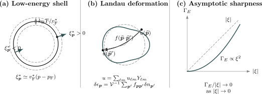
Landau theory resolves a weakly deformed Fermi surface into angular channels. The interaction function $f(\widehat{\mathbf p}\!\cdot\!\widehat{\mathbf p}')$ couples occupation changes at different surface points, while the quasiparticle width vanishes faster than the excitation energy near the surface.

Landau Kinetic Equation

Semiclassical evolution

Let

$$n_{\mathbf p\sigma} = n_{\mathbf p\sigma} (\mathbf r,t)$$

vary slowly in space and time. Its self-consistent quasiparticle energy is

$$\begin{aligned} \epsilon_{\mathbf p\sigma} (\mathbf r,t) ={}& \epsilon_{\mathbf p\sigma}^{*} + U_{\mathbf p\sigma} (\mathbf r,t) \\ & + \frac1{\mathcal V} \sum_{\mathbf p',\sigma'} f_{\mathbf p\sigma,\mathbf p'\sigma'} \\ & \qquad\times \delta n_{\mathbf p'\sigma'} (\mathbf r,t). \end{aligned}$$

The Landau kinetic equation is

$$\begin{aligned} \frac{\partial n_{\mathbf p\sigma}} {\partial t} & + \nabla_{\mathbf p} \epsilon_{\mathbf p\sigma} \cdot \nabla_{\mathbf r} n_{\mathbf p\sigma} \\ & - \nabla_{\mathbf r} \epsilon_{\mathbf p\sigma} \cdot \nabla_{\mathbf p} n_{\mathbf p\sigma} = I_{\mathrm{coll}} [n]. \end{aligned}$$

The streaming terms are Hamiltonian motion in phase space. The collision integral redistributes quasiparticles while respecting the exact conservation laws.

Boltzmann Transport owns the material band-distribution treatment, gain–loss kernels, electrical and thermal transport moments, and relaxation-time diagnostics. Here the kinetic equation additionally contains the self-consistent Landau interaction energy.

Linearized equation

Around a uniform equilibrium distribution,

$$\begin{aligned} \frac{\partial\delta n_{\mathbf p\sigma}} {\partial t} & + \mathbf v_{\mathbf p}^{*} \cdot \nabla_{\mathbf r} \delta n_{\mathbf p\sigma} \\ & - \nabla_{\mathbf r} \delta\epsilon_{\mathbf p\sigma} \cdot \nabla_{\mathbf p} n_{\mathbf p\sigma}^{0} = \delta I_{\mathrm{coll}}. \end{aligned}$$

For a plane wave,

$$\delta n_{\mathbf p} = - \frac{\partial n_{\mathrm F}} {\partial\epsilon} \nu(\widehat{\mathbf p}) e^{i(\mathbf q\cdot\mathbf r-\omega t)},$$

the collisionless equation becomes an angular integral equation on the Fermi surface.

Collisionless and hydrodynamic regimes

Let $\tau_{\mathrm{coll}}$ be the relevant local-equilibration time. Then

$$\omega\tau_{\mathrm{coll}} \gg 1$$

defines the collisionless regime, while

$$\omega\tau_{\mathrm{coll}} \ll 1$$

defines the hydrodynamic regime.

These limits can support different sound modes even in the same liquid:

• Hydrodynamic: local pressure and conservation laws provide the restoring description; the representative mode is first sound.
• Collisionless: a self-consistent Fermi-surface deformation provides the restoring description; the representative mode is zero sound.

Zero Sound

Simplest isotropic density model

Retain only the spin-symmetric $\ell=0$ parameter and take $\mathbf q$ along the polar axis. At zero temperature, define

$$s := \frac{\omega} {v_{\mathrm F}^{*}q}.$$

The collisionless integral equation can be written

$$\left( s-\cos\theta \right) \nu(\theta) = \cos\theta \left[ U + F_0^s \langle\nu\rangle \right],$$

where

$$\langle\nu\rangle := \frac12 \int_{-1}^{1} d(\cos\theta) \nu(\theta).$$

For a self-sustained mode, set $U=0$. Define

$$\Phi(s) := 1 - \frac{s}{2} \ln \left( \frac{s+1}{s-1} \right).$$

A nonzero angular average requires

$$1 + F_0^s \Phi(s) = 0, \qquad s>1.$$

The inequality $s>1$ places the phase velocity above the particle–hole continuum of the linearized isotropic model.

Weak repulsion

For

$$0 < F_0^s \ll1,$$

the solution lies exponentially close to the continuum edge:

$$s-1 \simeq 2 \exp \left[ -2 \left( 1+\frac1{F_0^s} \right) \right].$$

The mode is then delicate: curvature, finite temperature, disorder, or additional decay channels can matter.

Strong repulsion

For

$$F_0^s \gg1,$$

expand

$$\frac{s}{2} \ln \left( \frac{s+1}{s-1} \right) = 1 + \frac1{3s^2} + O(s^{-4}).$$

The zero-sound speed is therefore

$$s \simeq \sqrt{ \frac{F_0^s}{3} }.$$

Thus

$$\omega \simeq qv_{\mathrm F}^{*} \sqrt{ \frac{F_0^s}{3} }$$

in this asymptotic model.

Landau damping

For

$$\lvert s\rvert < 1,$$

the mode phase velocity overlaps quasiparticle velocities on the Fermi surface. The angular denominator

$$s-\cos\theta$$

then vanishes for some directions, producing an imaginary part of the response and collisionless Landau damping.

Being outside the simplest continuum suppresses this decay channel, but it does not guarantee an infinitely long lifetime. Multipair processes, impurities, lattice effects, and finite temperature can still attenuate the mode.

First-sound comparison

For a Galilean-invariant isotropic liquid, the hydrodynamic sound speed at zero temperature obeys

$$c_1^2 = \frac{n}{m} \frac{\partial\mu} {\partial n}.$$

Using the Landau compressibility,

$$c_1^2 = \frac{ v_{\mathrm F}^{*2} }{3} \frac{m^{*}}{m} \left( 1+F_0^s \right).$$

The first- and zero-sound formulas are different because local equilibrium is established in one regime and absent in the other.

Quasiparticle Lifetime

Phase-space suppression

A quasiparticle above the Fermi surface can decay by creating additional particle–hole excitations. Pauli blocking restricts all final fermions to narrow shells near the surface.

At zero temperature, two independent low-energy integrations give schematically

$$\Gamma_E(\xi,0) \sim \int_0^{\xi} d\epsilon_1 \int_0^{\xi-\epsilon_1} d\epsilon_2 \, \lvert\mathcal A\rvert^2.$$

Therefore, in a generic three-dimensional Fermi liquid,

$$\Gamma_E(\xi,0) \propto \xi^2.$$

The coefficient depends on scattering amplitudes, angular phase space, and the Fermi energy.

Finite-temperature scaling

The standard low-energy form is

$$\Gamma_E(\xi,T) = C \left[ \xi^2 + \pi^2 k_{\mathrm B}^2T^2 \right] + o(\xi^2,T^2),$$

where $C$ has dimensions of inverse energy and depends on the system and width convention.

Equivalently,

$$\tau_{\mathrm{pop}}^{-1} = \frac{C}{\hbar} \left[ \xi^2 + \pi^2 k_{\mathrm B}^2T^2 \right] + \cdots.$$

At zero temperature,

$$\frac{\Gamma_E(\xi,0)} {\lvert\xi\rvert} \propto \lvert\xi\rvert \longrightarrow 0.$$

This is the asymptotic sharpness criterion.

Thermal quasiparticles

For excitations in the thermal shell,

$$\lvert\xi\rvert \sim k_{\mathrm B}T,$$

the collision time scales as

$$\tau_{\mathrm{coll}} \propto T^{-2}$$

in a conventional three-dimensional Fermi liquid.

The collisionless condition becomes easier to satisfy as temperature falls:

$$\omega\tau_{\mathrm{coll}} \propto \omega T^{-2}.$$

This is why a liquid can cross from first-sound behavior to zero-sound behavior upon cooling at fixed probe frequency.

Two-dimensional qualification

In two dimensions, collinear and nearly forward kinematics can produce logarithmic corrections. A common zero-temperature scaling is

$$\Gamma_E(\xi,0) \sim \frac{\xi^2} {E_{\mathrm F}^{*}} \ln \left( \frac{E_{\mathrm F}^{*}} {\lvert\xi\rvert} \right)$$

up to channel-dependent coefficients.

The ratio still vanishes:

$$\frac{\Gamma_E} {\lvert\xi\rvert} \sim \frac{\lvert\xi\rvert} {E_{\mathrm F}^{*}} \ln \left( \frac{E_{\mathrm F}^{*}} {\lvert\xi\rvert} \right) \longrightarrow 0.$$

Thus a logarithm does not automatically destroy quasiparticles.

One-dimensional failure

In one dimension, the same fermion cannot generally remain an isolated pole after interactions are included. Spectral weight develops threshold power laws, and low-energy dynamics separates into collective charge and spin sectors.

The conventional criterion becomes

$$Z_{\mathrm F} = 0,$$

not merely a modified coefficient in the quadratic lifetime law. Luttinger Liquid Preview owns that alternative fixed point and its collective-boson description.

Lifetime Is Not Resistivity

Momentum conservation

Electron–electron collisions can produce

$$\tau_{\mathrm{qp}}^{-1} \propto T^2$$

while conserving total momentum exactly:

$$\sum_i \mathbf p_i^{\mathrm{in}} = \sum_i \mathbf p_i^{\mathrm{out}}.$$

In a clean Galilean-invariant one-component continuum,

$$\mathbf J = \frac{q}{m} \mathbf P,$$

so momentum-conserving collisions cannot relax the total electrical current.

Mechanisms that can relax current

A finite resistivity can require:

• Umklapp scattering on a lattice;
• impurities or boundaries;
• phonons or other momentum sinks;
• multiband current not proportional to total momentum;
• compensated electron and hole currents;
• explicit spatial inhomogeneity.

Therefore,

$$\rho(T) \propto T^2$$

is compatible with a Fermi liquid, but it is neither automatic nor a standalone proof.

Three distinct times

It is useful to separate:

$$\begin{aligned} \tau_{\mathrm{qp}} &: \text{single-particle spectral decay}, \\ \tau_{\mathrm{coll}} &: \text{local equilibration}, \\ \tau_{\mathrm{tr}} &: \text{current relaxation}. \end{aligned}$$

Forward scattering can strongly affect $\tau_{\mathrm{qp}}$ while weakly affecting $\tau_{\mathrm{tr}}$. Conserved angular harmonics can also make $\tau_{\mathrm{coll}}$ channel dependent.

Microscopic Matching

Self-energy data

A microscopic Green-function calculation can extract:

$$\begin{gathered} p_{\mathrm F}, \qquad Z_{\mathrm F}, \qquad v_{\mathrm F}^{*}, \\ \Gamma_E(\xi,T), \qquad \nu^{*}(0). \end{gathered}$$

The pole condition is

$$\xi_{\mathbf p}^{*} - \xi_{\mathbf p} - \operatorname{Re} \Sigma^{\mathrm R} \left( \mathbf p,\xi_{\mathbf p}^{*} \right) = 0.$$

The imaginary self-energy determines the intrinsic width only after the residue and width convention are included:

$$\Gamma_E = -2Z \operatorname{Im} \Sigma^{\mathrm R} \left( \mathbf p,\xi_{\mathbf p}^{*} \right).$$

Vertex data

The Landau interaction requires a renormalized four-point vertex in the appropriate forward limit. Schematically,

$$f \sim Z^2 \Gamma^{\omega} \quad \text{on the Fermi surface}.$$

The proportionality includes normalization and spin conventions. Computing only the self-energy does not determine every $F_{\ell}^{s,a}$ unless additional identities or approximations close the problem.

Ward identities

Charge, momentum, and spin conservation constrain the relation between:

• self-energy derivatives;
• current vertices;
• density vertices;
• Landau parameters;
• response sum rules.

An approximation that dresses propagators but omits the matching vertex correction can violate those constraints.

Diagrammatic Methods Preview owns the diagrammatic organization, while Green Functions in Many-Body QM owns the propagator framework.

Experimental and numerical extraction

Different observables constrain different combinations:

Observable	Primary low-energy information
heat capacity	$\nu^{*}(0)$ or a thermodynamic mass
quantum oscillation	extremal Fermi-surface area and cyclotron mass
photoemission	occupied dispersion, residue proxies, linewidth with matrix-element caveats
compressibility	$\nu^{*}(0)/(1+F_0^s)$
spin susceptibility	moment factors times $\nu^{*}(0)/(1+F_0^a)$
sound propagation	kinetic regime and combinations of Landau parameters
optical or dc transport	current vertex and momentum-relaxation mechanisms

No single measurement determines the entire Landau function.

Lattice, Multiband, and Anisotropic Generalizations

Fermi-surface integral

For a general Fermi surface, define its weighted measure by

$$d\mu_{\mathrm{FS}}(\mathbf p) := \frac{ dS_{\mathbf p} }{ (2\pi\hbar)^3 \lvert \mathbf v_{\mathrm F}^{*}(\mathbf p) \rvert }.$$

Then

$$\begin{gathered} \int \frac{d^3p} {(2\pi\hbar)^3} \delta \left( \xi_{\mathbf p}^{*} \right) (\cdots) \\ = \int_{\mathrm{FS}} d\mu_{\mathrm{FS}}(\mathbf p) (\cdots). \end{gathered}$$

The natural Landau function is then

$$f_{ab} \left( \mathbf p,\mathbf p' \right),$$

with $\mathbf p$ and $\mathbf p'$ restricted to Fermi-surface sheets and $a,b$ denoting band, orbital, or pseudospin indices.

Crystal harmonics

Spherical harmonics should be replaced by basis functions transforming under the crystal point group:

$$\phi_{\Gamma,\alpha} \left( \mathbf p \right).$$

A deformation is expanded as

$$u_a(\mathbf p) = \sum_{\Gamma,\alpha} u_{\Gamma,\alpha,a} \phi_{\Gamma,\alpha} (\mathbf p).$$

Stability is then an eigenvalue problem for an integral kernel rather than the scalar inequality

$$F_{\ell}>-(2\ell+1).$$

Multiple sheets

In a multiband metal, a uniform density perturbation can transfer particles between sheets. The compressibility and spin response involve matrices:

$$\boldsymbol{\chi} \sim \left( \boldsymbol{\nu}^{*-1} + \mathbf f \right)^{-1}.$$

Interband drag, orbital matrix elements, and sheet-dependent lifetimes become essential.

Spin-orbit coupling

When spin is not conserved, the separation into $s$ and $a$ channels is not exact. The interaction function is a matrix in pseudospin space, and magnetic response depends on both quasiparticle moments and interband contributions.

The Landau strategy still applies: identify the low-energy surface labels, write the most general symmetry-allowed energy functional, and diagonalize its response channels.

What Counts as Evidence

Strong combined evidence

A conventional Fermi-liquid interpretation is strongest when several observations agree:

1. A stable Fermi surface is identified.
2. The single-particle spectrum contains a pole-like branch with $Z_{\mathrm F}>0$.
3. The width satisfies $\Gamma_E/\lvert\xi\rvert\to0$.
4. Low-temperature heat capacity is linear with a stable coefficient.
5. Static responses are mutually consistent with a set of Landau parameters.
6. Collisionless and hydrodynamic regimes follow the expected time-scale ordering.
7. Sum rules and conservation laws are respected.
8. No lower-temperature ordered phase intervenes in the claimed window.

Evidence that is insufficient alone

None of the following proves a Landau Fermi liquid by itself:

• a Fermi-surface-like contour;
• a linear heat capacity over a narrow range;
• a $T^2$ resistivity;
• a peak fitted by a Lorentzian;
• a finite effective mass;
• agreement with one static susceptibility;
• perturbatively weak bare interactions;
• the absence of obvious symmetry breaking.

Each can also occur, approximately or accidentally, in a broader class of systems.

Scaling window

Real systems are never measured at exactly

$$\xi = T = q = \omega = 0.$$

One should state a window such as

$$\max \left( \lvert\xi\rvert, k_{\mathrm B}T, \hbar\omega, \hbar v_{\mathrm F}^{*}q \right) \ll E_{\mathrm{FL}},$$

where $E_{\mathrm{FL}}$ is the crossover scale below which Fermi-liquid scaling is observed.

A small $E_{\mathrm{FL}}$ can make a conventional asymptotic fixed point experimentally difficult to distinguish from an extended crossover.

Breakdown and Competing Infrared Physics

Pairing

An attractive Cooper channel is marginally unstable in the idealized normal Fermi liquid. Below a transition scale, the appropriate low-energy excitations are Bogoliubov quasiparticles and collective phase modes rather than normal-state Landau quasiparticles at a gapless surface.

BCS Mean-Field Theory develops that saddle.

One dimension

One-dimensional phase space enhances collective fluctuations. Fermionic residue vanishes and correlation functions exhibit interaction-dependent power laws. A pair of Fermi points remains meaningful, but the low-energy fixed point is a Luttinger liquid rather than a Landau Fermi liquid.

Quantum criticality

Near a quantum critical point, scattering from soft order-parameter fluctuations can generate

$$\Gamma_E(\xi) \not\ll \lvert\xi\rvert.$$

The residue may vanish, the effective mass may become singular, or only selected regions of the Fermi surface may remain coherent.

Gauge fields and fractionalization

Emergent gauge fields can couple singularly to a Fermi surface. The electron may fractionalize into partons, or a neutral Fermi surface may appear without electron-like quasiparticles.

The existence of a surface of gapless excitations then does not imply the electron Green function has a Landau pole.

Non-Fermi Liquids classifies these and other replacement infrared theories and gives the material evidence workflow for distinguishing them.

Mott physics

At a Mott transition, charge localization can destroy the adiabatic connection to a free electron gas even without a simple weak-coupling band gap. Spectral weight can transfer over microscopic energy scales, making a low-order quasiparticle expansion insufficient.

Disorder

Weak disorder broadens momentum while a diffusive interacting metal can still retain quasiparticle thermodynamics. Strong disorder, localization, or rare-region physics can invalidate the homogeneous kinetic description.

Ordered Fermi surfaces

Magnetism, density waves, or nematic order may reconstruct the Fermi surface. The resulting phase can itself be a Fermi liquid of reconstructed bands, but it is not adiabatically connected to the original symmetric state without crossing an ordering transition.

Worked Example: Extracting Two Landau Parameters

Suppose a three-dimensional isotropic system at fixed density has

$$\frac{\gamma}{\gamma_0} = 2.5, \qquad \frac{\kappa}{\kappa_0} = 1.25, \qquad \frac{\chi}{\chi_0} = 5.$$

Assuming an unchanged quasiparticle magnetic moment and Galilean invariance,

$$\frac{m^{*}}{m} = 2.5.$$

The compressibility ratio gives

$$1.25 = \frac{2.5} {1+F_0^s},$$

so

$$F_0^s = 1.$$

The spin ratio gives

$$5 = \frac{2.5} {1+F_0^a},$$

so

$$F_0^a = -0.5.$$

Both $\ell=0$ channels are stable:

$$1+F_0^s = 2 > 0, \qquad 1+F_0^a = 0.5 > 0.$$

The enhanced spin response comes partly from the heavier quasiparticle density of states and partly from an attractive spin-antisymmetric Landau channel.

Worked Example: Sharpness Scale

Let a measured intrinsic width follow

$$\Gamma_E(\xi,0) = \frac{\xi^2} {20\,\mathrm{meV}}$$

within a low-energy window.

At

$$\lvert\xi\rvert = 2\,\mathrm{meV},$$

the width is

$$\Gamma_E = 0.2\,\mathrm{meV}.$$

The sharpness ratio is

$$\frac{\Gamma_E} {\lvert\xi\rvert} = 0.1.$$

At

$$\lvert\xi\rvert = 0.5\,\mathrm{meV},$$

one finds

$$\Gamma_E = 0.0125\,\mathrm{meV},$$

and

$$\frac{\Gamma_E} {\lvert\xi\rvert} = 0.025.$$

The absolute width narrows, but the decisive feature is that it narrows faster than the excitation energy.

Common Mistakes

Equating Fermi surface with Fermi liquid

A Fermi surface is a momentum-space singular structure. A Landau Fermi liquid additionally requires long-lived quasiparticles and a regular low-energy energy functional.

Treating adiabatic continuity as weak coupling

The interacting wavefunction can be highly correlated. The claim concerns low-energy state organization, not a small bare coupling.

Setting effective mass equal to inverse residue

The relation

$$\frac{m^{*}}{m} = \frac1Z$$

holds only in special approximations with negligible momentum dependence of the self-energy. It is not a general identity.

Ignoring density-of-states conventions

Using a per-spin $\nu^{*}(0)$ with total-spin formulas changes every $F_{\ell}^{s,a}$ by a factor of two.

Applying the Galilean mass relation on a lattice

The identity

$$\frac{m^{*}}{m} = 1+\frac{F_1^s}{3}$$

requires continuous boost invariance and the stated three-dimensional convention.

Calling every forward interaction a Landau parameter

Bare Coulomb matrix elements, screened static interactions, scattering amplitudes, and Landau functions are related but not identical objects.

Reading a displayed width as an intrinsic rate

Instrumental resolution, finite-size broadening, and numerical $\eta$ do not establish a quasiparticle lifetime.

Inferring resistivity from the quasiparticle rate

Momentum-conserving collisions can broaden a single-particle pole without relaxing the total current.

Forgetting order of limits

Static thermodynamics, collisionless response, and transport can take different paths through

$$(\mathbf q,\omega,T) \to (0,0,0).$$

Truncating angular channels without checking stability

An $\ell=0$ model cannot diagnose an $\ell=2$ nematic instability or an anisotropic lattice eigenmode.

Using three-dimensional scaling in one dimension

The one-dimensional infrared fixed point is qualitatively different; it is not obtained by changing one numerical exponent in a quasiparticle width.

Practical Analysis Workflow

1. Identify the low-energy surface. Determine its sheets, symmetry, dimensionality, and relevant conserved quantum numbers.
2. Fix conventions. State whether momentum is $\mathbf p$ or $\mathbf k$, whether the density of states is total or per spin, and how linewidth is defined.
3. Test the pole. Extract dispersion, residue, intrinsic width, and incoherent background from a controlled spectral analysis.
4. Check asymptotic sharpness. Test $\Gamma_E/\lvert\xi\rvert\to0$ and separate the $\xi$ and $T$ limits.
5. Measure thermodynamic mass. Use heat capacity or another density-of-states probe within a demonstrated low-temperature window.
6. Extract response combinations. Combine compressibility and spin response with the mass to infer $F_0^s$ and $F_0^a$ under stated assumptions.
7. Check symmetry identities. Apply the $F_1^s$ mass relation only when Galilean invariance is present.
8. Test stability. Examine all symmetry-allowed deformation channels, not only uniform ones.
9. Separate kinetic regimes. Compare $\omega\tau_{\mathrm{coll}}$ with unity before naming first or zero sound.
10. Audit transport relaxation. Identify the mechanism that transfers momentum out of the current-carrying sector.
11. Look for competing order. Pairing, magnetism, density waves, and criticality can truncate the normal-state scaling window.
12. Cross-check observables. A credible Landau parameter set should explain more than one measurement and respect conservation laws.

Exercises

Exercise 1: Functional derivative

Starting from

$$\begin{aligned} \delta E ={}& \sum_a \epsilon_a^{*} \delta n_a \\ & + \frac1{2\mathcal V} \sum_{a,b} f_{ab} \delta n_a \delta n_b, \end{aligned}$$

where $a=(\mathbf p,\sigma)$, derive the shift of the quasiparticle energy. State the symmetry required of $f_{ab}$.

Solution

Differentiate with respect to $\delta n_c$:

$$\begin{aligned} \frac{\partial\delta E} {\partial\delta n_c} ={}& \epsilon_c^{*} \\ & + \frac1{2\mathcal V} \sum_b f_{cb} \delta n_b \\ & + \frac1{2\mathcal V} \sum_a f_{ac} \delta n_a. \end{aligned}$$

Because the interaction function is a second derivative of the energy,

$$f_{ab} = f_{ba}.$$

The last two sums are equal, giving

$$\widetilde\epsilon_c = \epsilon_c^{*} + \frac1{\mathcal V} \sum_b f_{cb} \delta n_b.$$

Therefore

$$\delta\epsilon_c = \frac1{\mathcal V} \sum_b f_{cb} \delta n_b.$$

The factor $1/2$ prevents double counting in the energy but disappears from its first derivative.

Exercise 2: Heat-capacity mass

An isotropic three-dimensional Fermi liquid has a measured low-temperature coefficient

$$\gamma = 3\gamma_0.$$

Under Galilean-invariant single-band assumptions, find $m^{*}/m$ and $F_1^s$.

Solution

At fixed density,

$$\frac{\gamma}{\gamma_0} = \frac{\nu^{*}(0)}{\nu_0(0)} = \frac{m^{*}}{m}.$$

Hence

$$\frac{m^{*}}{m} = 3.$$

Galilean invariance gives

$$3 = 1+\frac{F_1^s}{3}.$$

Therefore

$$F_1^s = 6.$$

On a lattice the first conclusion may define a thermodynamic mass ratio relative to a chosen band benchmark, but the second conclusion does not follow.

Exercise 3: Asymptotic sharpness

Suppose

$$\Gamma_E(\xi,0) = \alpha \frac{\xi^2} {E_{\mathrm F}^{*}}$$

with dimensionless $\alpha>0$. Show that the quasiparticle becomes asymptotically sharp. How many oscillation periods fit into the population lifetime, up to factors of $2\pi$?

Solution

The sharpness ratio is

$$\frac{\Gamma_E} {\lvert\xi\rvert} = \alpha \frac{\lvert\xi\rvert} {E_{\mathrm F}^{*}} \longrightarrow 0.$$

The population lifetime is

$$\tau_{\mathrm{pop}} = \frac{\hbar}{\Gamma_E}.$$

The characteristic oscillation time associated with the excitation energy is

$$t_{\xi} \sim \frac{\hbar}{\lvert\xi\rvert}.$$

Their ratio is

$$\frac{\tau_{\mathrm{pop}}}{t_{\xi}} \sim \frac{\lvert\xi\rvert}{\Gamma_E} = \frac{E_{\mathrm F}^{*}} {\alpha\lvert\xi\rvert} \longrightarrow \infty.$$

Thus the excitation completes parametrically many cycles before its population decays. Counting full $2\pi$ periods inserts an additional factor $1/(2\pi)$ without changing the divergence.

Exercise 4: Compressibility and stability

For

$$\frac{m^{*}}{m} = 2, \qquad F_0^s = -0.8,$$

find $\kappa/\kappa_0$. Is the uniform density channel stable?

Solution

The ratio is

$$\frac{\kappa}{\kappa_0} = \frac{2}{1-0.8} = 10.$$

Uniform density stability requires

$$1+F_0^s > 0.$$

Here

$$1+F_0^s = 0.2 > 0,$$

so the channel is stable but close to an $\ell=0$ symmetric instability. The large compressibility reflects that proximity.

Exercise 5: Spin response

A Fermi liquid has

$$\frac{\gamma}{\gamma_0} = 4, \qquad \frac{\chi}{\chi_0} = 8.$$

Assuming unchanged moment factors, find $F_0^a$ and the Wilson ratio.

Solution

The response formula gives

$$8 = \frac{4}{1+F_0^a}.$$

Therefore

$$1+F_0^a = \frac12,$$

and

$$F_0^a = -\frac12.$$

The normalized Wilson ratio is

$$R_{\mathrm W} = \frac{8}{4} = 2.$$

Equivalently,

$$R_{\mathrm W} = \frac1{1+F_0^a} = 2.$$

Exercise 6: Pomeranchuk threshold

Find the stability boundary for a spin-symmetric quadrupolar deformation in three dimensions. What qualitative shape change does it represent?

Solution

A quadrupolar deformation has

$$\ell = 2.$$

The stability criterion is

$$1 + \frac{F_2^s}{5} > 0.$$

Therefore the boundary is

$$F_2^s = -5.$$

At the boundary, an $\ell=2$ spin-symmetric shape mode becomes soft. In an isotropic continuum this is a quadrupolar distortion of the Fermi surface. In a crystal, the corresponding components split into point-group representations and can describe an electronic nematic instability.

Exercise 7: Strong-coupling zero sound

Starting from

$$1 + F_0^s \left[ 1 - \frac{s}{2} \ln \left( \frac{s+1}{s-1} \right) \right] = 0,$$

derive the leading large-$F_0^s$ result for $s$.

Solution

For $s\gg1$,

$$\ln \left( \frac{s+1}{s-1} \right) = 2 \left[ \frac1s + \frac1{3s^3} + O(s^{-5}) \right].$$

Hence

$$\frac{s}{2} \ln \left( \frac{s+1}{s-1} \right) = 1 + \frac1{3s^2} + O(s^{-4}).$$

The mode equation becomes

$$1 - \frac{F_0^s}{3s^2} + O \left( \frac{F_0^s}{s^4} \right) = 0.$$

To leading order,

$$s^2 = \frac{F_0^s}{3},$$

so

$$s \simeq \sqrt{ \frac{F_0^s}{3} }.$$

Exercise 8: Why collisions need not cause resistivity

Show why a finite electron–electron collision rate does not produce finite dc resistivity in a clean Galilean-invariant one-component continuum.

Solution

Galilean invariance ties total current to conserved total momentum:

$$\mathbf J = \frac{q}{m} \mathbf P.$$

Translation-invariant two-body collisions conserve momentum:

$$\frac{d\mathbf P}{dt} = 0.$$

Therefore

$$\frac{d\mathbf J}{dt} = \frac{q}{m} \frac{d\mathbf P}{dt} = 0$$

in the absence of external momentum relaxation.

The same collisions can redistribute occupation around the Fermi surface and broaden a single-particle pole, so

$$\tau_{\mathrm{qp}}^{-1} > 0$$

is possible while

$$\tau_{\mathrm{tr}}^{-1} = 0.$$

A lattice Umklapp process, impurity, boundary, phonon bath, or other momentum sink is needed to obtain finite dc resistivity in this idealized setting.

Cross-Links

• Fermi Surface for geometry, Fermi velocity, occupation singularities, and volume relations.
• Quasiparticles Overview for the general quasiparticle definition, pole tests, dressing, and breakdown.
• Particle–Hole Excitations for particle–hole states, continua, and response support.
• Spectral Functions for residue, coherent weight, linewidth, lifetime, and experimental-intensity conventions.
• Green Functions in Many-Body QM for Dyson equations and propagator structure.
• Susceptibilities for static and dynamic source conventions.
• Collective Modes for response poles, damping, hybridization, and mode classification.
• Itinerant Magnetism for the material realization of spin-polarized quasiparticle bands, magnetic instabilities, and collective modes embedded in particle–hole continua.
• Heavy Fermions for the multiband materials diagnosis of strongly renormalized quasiparticles, coherence scales, and the limits of a single effective mass.
• Stoner Criterion for the scalar energy-curvature derivation and its convention-aware relation to the $F_0^a=-1$ boundary.
• Transport Coefficients Preview for current relaxation, Drude weight, diffusion, and hydrodynamic limits.
• Diagrammatic Methods Preview for self-energy and vertex approximations.
• Degenerate Fermi Gas for the ideal-gas thermal shell and Pauli-blocking baseline.
• Low-Dimensional Quantum Gases for dimensional state counting and one-dimensional kinematics.
• Condensed Matter Roadmap for a broader study sequence.

References

1. L. D. Landau, “The Theory of a Fermi Liquid,” Soviet Physics JETP 3, 920–925 (1957), translated from Zh. Eksp. Teor. Fiz. 30, 1058–1064 (1956). JETP article.
2. L. D. Landau, “Oscillations in a Fermi Liquid,” Soviet Physics JETP 5, 101–108 (1957), translated from Zh. Eksp. Teor. Fiz. 32, 59–66 (1957). JETP article.
3. A. A. Abrikosov and I. M. Khalatnikov, “The Theory of a Fermi Liquid,” Reports on Progress in Physics 22, 329–367 (1959). doi:10.1088/0034-4885/22/1/310.
4. D. Pines and P. Nozières, The Theory of Quantum Liquids, Volume I: Normal Fermi Liquids, W. A. Benjamin (1966).
5. P. Nozières, Theory of Interacting Fermi Systems, W. A. Benjamin (1964).
6. G. Baym and C. Pethick, Landau Fermi-Liquid Theory: Concepts and Applications, Wiley-VCH (1991). doi:10.1002/9783527617159.
7. A. J. Leggett, “A Theoretical Description of the New Phases of Liquid $^3\mathrm{He}$,” Reviews of Modern Physics 47, 331–414 (1975). doi:10.1103/RevModPhys.47.331.
8. J. M. Luttinger, “Fermi Surface and Some Simple Equilibrium Properties of a System of Interacting Fermions,” Physical Review 119, 1153–1163 (1960). doi:10.1103/PhysRev.119.1153.
9. A. A. Abrikosov, L. P. Gor’kov, and I. E. Dzyaloshinski, Methods of Quantum Field Theory in Statistical Physics, Dover (1975).
10. E. M. Lifshitz and L. P. Pitaevskii, Statistical Physics, Part 2, Butterworth-Heinemann (1980).
11. G. F. Giuliani and G. Vignale, Quantum Theory of the Electron Liquid, Cambridge University Press (2005). doi:10.1017/CBO9780511619915.
12. R. Shankar, “Renormalization-Group Approach to Interacting Fermions,” Reviews of Modern Physics 66, 129–192 (1994). doi:10.1103/RevModPhys.66.129.
13. F. D. M. Haldane, “‘Luttinger Liquid Theory’ of One-Dimensional Quantum Fluids,” Journal of Physics C 14, 2585–2609 (1981). doi:10.1088/0022-3719/14/19/010.
14. C. M. Varma, P. B. Littlewood, S. Schmitt-Rink, E. Abrahams, and A. E. Ruckenstein, “Phenomenology of the Normal State of Cu–O High-Temperature Superconductors,” Physical Review Letters 63, 1996–1999 (1989). doi:10.1103/PhysRevLett.63.1996.
15. P. Wölfle, “Quasiparticles in Condensed Matter Systems,” Reports on Progress in Physics 81, 032501 (2018). doi:10.1088/1361-6633/aa9bc4.
16. A. V. Chubukov, D. L. Maslov, and A. J. Millis, “Nonanalytic Corrections to the Specific Heat of a Three-Dimensional Fermi Liquid,” Physical Review B 73, 045128 (2006). doi:10.1103/PhysRevB.73.045128.
17. C. Hodges, H. Smith, and J. W. Wilkins, “Effect of Fermi Surface Geometry on Electron-Electron Scattering,” Physical Review B 4, 302–311 (1971). doi:10.1103/PhysRevB.4.302.