Polarons Preview

A polaron is a mobile microscopic particle dressed by excitations and correlations of its environment. The particle and its surrounding response propagate as one composite quasiparticle when the dressed branch is sufficiently sharp.

The word describes a physical organization, not one Hamiltonian. The moving object may be

• an electron accompanied by a lattice-polarization cloud;
• a minority atom moving through a Fermi sea;
• an impurity immersed in a Bose–Einstein condensate;
• a hole dressed by spin fluctuations in a magnet;
• or another mobile degree of freedom coupled to a deformable medium.

Across these realizations, the same questions recur:

$$\begin{gathered} \text{Energy lowering?} \\ \text{Dispersion and effective mass?} \\ \text{Bare-particle overlap?} \\ \text{Cloud correlations?} \\ \text{Stability and decay?} \end{gathered}$$

A cloud is not an extra rigid object glued to the particle. It is a pattern of conditional correlations in the host. In a translation-invariant momentum eigenstate, the one-point density is uniform even though the density around a detected impurity is strongly distorted.

Scope and Canonical Ownership

This page owns the generic mobile-impurity framework:

• a particle linearly coupled to bosonic environmental modes;
• conservation of total momentum and the Lee–Low–Pines transformation;
• exact static-impurity and weak-coupling benchmarks;
• polaron energy, dispersion, effective mass, residue, cloud observables, and lifetime;
• kinematic emission thresholds;
• Fröhlich and Holstein electron–phonon models as complementary examples;
• Fermi-polaron and Bose-polaron constructions;
• attractive, repulsive, molecular, and continuum branches;
• common approximation strategies and their domains;
• failure of the finite-residue quasiparticle picture.

Neighboring pages retain their canonical subjects:

• Quasiparticles Overview owns the general pole, residue, lifetime, and quasiparticle taxonomy.
• Spectral Functions owns spectral normalization, sum rules, linewidth conventions, and experimental forward models.
• Green Functions in Many-Body QM owns Lehmann representations and the full Dyson construction.
• Phonons as Many-Body Excitations owns lattice normal modes and their quantization.
• Bogoliubov Theory owns the diagonalization of weak-condensate host fluctuations.
• Displaced Oscillator owns the exact one-mode displacement algebra used in the static benchmark.
• Particle–Hole Excitations owns Fermi-sea particle–hole kinematics.
• Anderson Impurity Model Preview owns a localized correlated orbital hybridized with a bath. A polaron impurity is mobile, so recoil and total momentum are essential.
• Effective Mass owns the general curvature formula.

Detailed small- and large-polaron material phenomenology, optical conductivity, first-principles electron–phonon matrix elements, transport, and superconducting pairing route through the Lattice Vibrations and Collective Modes gateway to their material and probe owners. Here those subjects appear only far enough to establish the dressed-particle framework.

Convention Ledger

Several otherwise correct formulas look inconsistent when momentum and Fourier conventions are mixed. This page uses the following ledger unless a subsection says otherwise.

• Bold uppercase $\mathbf P$ denotes a physical momentum.
• Bold lowercase $\mathbf q$ denotes a wave vector, so one host quantum carries momentum $\hbar\mathbf q$.
• The system is first placed in a finite periodic volume $\mathcal V$; sums become integrals only after normalization is fixed.
• The coefficient $V_{\mathbf q}$ includes the chosen Fourier-volume factor.
• The bare mobile particle has mass $M$ and position $\hat{\mathbf R}$.
• Host bosonic modes obey

$$[b_{\mathbf q},b_{\mathbf q'}^\dagger] = \delta_{\mathbf q\mathbf q'}.$$

• Their energies are $\hbar\omega_{\mathbf q}>0$.
• A retarded Green function is written as a function of energy $E$, not angular frequency.

For a continuum sum,

$$\frac1{\mathcal V} \sum_{\mathbf q} \longrightarrow \int\frac{d^dq}{(2\pi)^d}.$$

Whether $1/\sqrt{\mathcal V}$ is shown explicitly in $V_{\mathbf q}$ or absorbed into it is conventional. Physical energy shifts must remain intensive.

Dressing as a Change of the Excitation

Bare particle versus dressed eigenstate

Let $a_{\mathbf P}^\dagger|0\rangle$ denote a state in which a microscopic particle has been inserted with no host excitations. Once the interaction is present, this state is generally not an eigenstate. It overlaps a family of exact states containing different host configurations:

$$a_{\mathbf P}^\dagger|0\rangle = \sum_n \langle\Psi_{n\mathbf P}| a_{\mathbf P}^\dagger|0\rangle |\Psi_{n\mathbf P}\rangle.$$

If one overlap is associated with an isolated low-energy branch, that branch can be called a polaron. Schematically,

$$\begin{aligned} |\Psi_{\mathbf P}^{\mathrm{pol}}\rangle ={}& \sqrt{Z_{\mathbf P}}|\mathrm{bare}\rangle \\ &+ |\mathrm{cloud}\rangle_\perp, \end{aligned}$$

where the two terms are orthogonal and $0\le Z_{\mathbf P}\le1$ for a normalized state. The label $|\mathrm{cloud}\rangle_\perp$ includes both the particle and its orthogonal host-excitation sectors; it can contain one excitation, many excitations, particle–hole pairs, bound clusters, or nonperturbative host rearrangement.

The bare particle has not disappeared. Rather, it is no longer the variable that diagonalizes long-time propagation.

The cloud is relational

Suppose $n_I(\mathbf r)$ and $n_B(\mathbf r)$ are impurity and bath densities. In a translation-invariant one-polaron momentum eigenstate,

$$\langle n_I(\mathbf r)\rangle = \frac1{\mathcal V},$$

and the host one-point density is also uniform. A useful cloud profile is instead conditional:

$$\delta n_{B|I}(\mathbf r) = \frac{ \langle n_I(\mathbf 0)n_B(\mathbf r)\rangle }{ \langle n_I(\mathbf 0)\rangle } -n_B.$$

This asks how the host density differs from its bulk value given that the impurity is found at the origin.

Three quantities must not be identified without a derivation:

1. the integrated density excess or depletion around the impurity;
2. the number of quasibosons $\sum_{\mathbf q}\langle b_{\mathbf q}^\dagger b_{\mathbf q}\rangle$;
3. the loss of bare-particle residue $1-Z$.

They probe different decompositions of the same state. A Bogoliubov quasiboson is not literally one displaced host atom, and a small residue need not imply a large integrated density excess.

Generic Mobile Impurity Coupled to Bosons

Hamiltonian

A broad class of polaron models begins with

$$\begin{aligned} H={}& \frac{\hat{\mathbf P}^{\,2}}{2M} + \sum_{\mathbf q} \hbar\omega_{\mathbf q} b_{\mathbf q}^\dagger b_{\mathbf q} \\ &+ \sum_{\mathbf q} \left( V_{\mathbf q} e^{i\mathbf q\cdot\hat{\mathbf R}} b_{\mathbf q} + V_{\mathbf q}^* e^{-i\mathbf q\cdot\hat{\mathbf R}} b_{\mathbf q}^\dagger \right). \end{aligned}$$

The exponential transfers momentum between the mobile particle and the host. The interaction annihilates or creates one host quantum while preserving total momentum.

This linear boson model can be fundamental over a restricted regime or can arise after expanding a more microscopic interaction around an equilibrium background. Its simplicity should not be mistaken for universality at strong coupling. Terms quadratic and higher in host fluctuations may matter.

Conserved total momentum

Define the host momentum

$$\hat{\mathbf P}_{\mathrm b} = \sum_{\mathbf q} \hbar\mathbf q\, b_{\mathbf q}^\dagger b_{\mathbf q},$$

and total momentum

$$\hat{\mathbf P}_{\mathrm{tot}} = \hat{\mathbf P} + \hat{\mathbf P}_{\mathrm b}.$$

For the translation-invariant Hamiltonian,

$$[H,\hat{\mathbf P}_{\mathrm{tot}}]=0.$$

The interaction does not conserve the impurity momentum or host momentum separately. If a boson of wave vector $\mathbf q$ is created, the impurity recoils by $-\hbar\mathbf q$.

The conserved label of a polaron branch is therefore total momentum, not the instantaneous momentum carried by the microscopic particle.

What the model omits

The minimal Hamiltonian omits, unless encoded effectively in its parameters,

• host–host interactions beyond the chosen normal modes;
• two-boson scattering from the impurity;
• internal impurity structure;
• lattice Umklapp and band geometry;
• disorder and boundaries;
• finite impurity concentration;
• irreversible driving and loss.

Every application should state why these omissions are controlled or at least quantitatively modest.

Lee–Low–Pines Frame

Removing the impurity coordinate

Translation invariance permits an exact change of frame. Define

$$\mathcal U_{\mathrm{LLP}} = \exp\!\left( -\frac{i}{\hbar} \hat{\mathbf R}\cdot \hat{\mathbf P}_{\mathrm b} \right),$$

and transform operators and the Hamiltonian according to

$$\widetilde H = \mathcal U_{\mathrm{LLP}}^\dagger H \mathcal U_{\mathrm{LLP}}.$$

The useful identities are

$$\mathcal U_{\mathrm{LLP}}^\dagger \hat{\mathbf P} \mathcal U_{\mathrm{LLP}} = \hat{\mathbf P}-\hat{\mathbf P}_{\mathrm b},$$ $$\mathcal U_{\mathrm{LLP}}^\dagger b_{\mathbf q} \mathcal U_{\mathrm{LLP}} = e^{-i\mathbf q\cdot\hat{\mathbf R}} b_{\mathbf q},$$

and

$$\mathcal U_{\mathrm{LLP}}^\dagger \hat{\mathbf P}_{\mathrm{tot}} \mathcal U_{\mathrm{LLP}} = \hat{\mathbf P}.$$

The transformed impurity momentum operator is the conserved total momentum. In its eigen-sector with value $\mathbf P$,

$$\begin{aligned} \widetilde H_{\mathbf P} ={}& \frac{ (\mathbf P-\hat{\mathbf P}_{\mathrm b})^2 }{2M} + \sum_{\mathbf q} \hbar\omega_{\mathbf q} b_{\mathbf q}^\dagger b_{\mathbf q} \\ &+ \sum_{\mathbf q} \left( V_{\mathbf q}b_{\mathbf q} +V_{\mathbf q}^*b_{\mathbf q}^\dagger \right). \end{aligned}$$

The impurity coordinate has disappeared. The price is the recoil term

$$\frac{\hat{\mathbf P}_{\mathrm b}^{\,2}}{2M},$$

which couples bosonic modes even when the original host Hamiltonian was diagonal.

Physical interpretation

The Lee–Low–Pines frame follows the mobile particle while retaining total momentum as a parameter. It makes several facts transparent:

• host quanta share the conserved momentum with the microscopic particle;
• finite impurity mass correlates different host modes through recoil;
• the static-impurity limit removes that recoil coupling;
• a coherent-state ansatz can describe a momentum-dependent dressing cloud without localizing the total state.

The transformation is exact. Approximations begin only when one chooses a restricted state, truncates interactions, or evaluates the transformed Hamiltonian perturbatively.

Exact Static-Impurity Benchmark

Independent displaced modes

As $M\to\infty$, recoil vanishes. Apart from a constant bare impurity energy,

$$H_\infty = \sum_{\mathbf q} \left[ \hbar\omega_{\mathbf q} b_{\mathbf q}^\dagger b_{\mathbf q} +V_{\mathbf q}b_{\mathbf q} +V_{\mathbf q}^*b_{\mathbf q}^\dagger \right].$$

For every mode define

$$c_{\mathbf q} = b_{\mathbf q} + \frac{V_{\mathbf q}^*} {\hbar\omega_{\mathbf q}}.$$

Then

$$H_\infty = \sum_{\mathbf q} \hbar\omega_{\mathbf q} c_{\mathbf q}^\dagger c_{\mathbf q} - \sum_{\mathbf q} \frac{|V_{\mathbf q}|^2} {\hbar\omega_{\mathbf q}}.$$

The exact dressing energy is

$$\Delta E_\infty = -\sum_{\mathbf q} \frac{|V_{\mathbf q}|^2} {\hbar\omega_{\mathbf q}}.$$

It is nonpositive for stable positive-frequency modes. The environment relaxes around the static source and lowers the energy.

Cloud occupation and bare overlap

The exact ground state is a product of coherent states of the original $b_{\mathbf q}$ modes, with amplitudes

$$\alpha_{\mathbf q} = -\frac{V_{\mathbf q}^*} {\hbar\omega_{\mathbf q}}.$$

Its mean boson number is

$$N_{\mathrm b} = \sum_{\mathbf q} |\alpha_{\mathbf q}|^2 = \sum_{\mathbf q} \frac{|V_{\mathbf q}|^2} {(\hbar\omega_{\mathbf q})^2}.$$

The amplitude overlap with the undistorted boson vacuum is

$$\langle0|\{\alpha_{\mathbf q}\}\rangle = e^{-N_{\mathrm b}/2} e^{i\varphi},$$

so the squared overlap is

$$Z_\infty=e^{-N_{\mathrm b}}.$$

This exact relation is special to the coherent-product static problem. In a generic interacting polaron, $Z$ cannot be inferred from a boson number alone.

Infrared convergence

Energy and overlap test different integrals. In a continuum,

$$|\Delta E_\infty| \sim \int d^dq\, \frac{|V_{\mathbf q}|^2} {\hbar\omega_{\mathbf q}},$$

whereas

$$-\ln Z_\infty \sim \int d^dq\, \frac{|V_{\mathbf q}|^2} {(\hbar\omega_{\mathbf q})^2}.$$

The energy integral may converge while the overlap integral diverges. Then inserting the impurity costs a finite energy, but the dressed and bare vacua become orthogonal in the thermodynamic limit:

$$Z_\infty\to0.$$

This is an orthogonality catastrophe, not an infinite dressing energy. It warns that finite energy does not guarantee a finite-residue quasiparticle pole.

Weak-Coupling Mobile Benchmark

Second-order energy

At total momentum $\mathbf P=\mathbf0$, the unperturbed state contains no host bosons. A one-boson virtual state of wave vector $\mathbf q$ has excitation cost

$$D_{\mathbf q} = \hbar\omega_{\mathbf q} + \frac{\hbar^2q^2}{2M}.$$

The second term is impurity recoil. Nondegenerate second-order perturbation theory gives

$$E_0^{(2)} = -\sum_{\mathbf q} \frac{|V_{\mathbf q}|^2}{D_{\mathbf q}}.$$

For $M\to\infty$, this approaches the leading term of the exact displaced-mode answer. At finite $M$, recoil increases the denominator and reduces the magnitude of the energy lowering.

The leading one-boson amplitude is

$$\alpha_{\mathbf q}^{(1)} = -\frac{V_{\mathbf q}^*}{D_{\mathbf q}}.$$

After normalizing the state,

$$1-Z_0 = \sum_{\mathbf q} \frac{|V_{\mathbf q}|^2}{D_{\mathbf q}^2} +O(V^4).$$

Energy and residue again involve different powers of the denominator.

Momentum-dependent energy

For small total momentum, define the recoil denominator

$$\Delta_{\mathbf q}(\mathbf P) = D_{\mathbf q} - \frac{\mathbf P\cdot\hbar\mathbf q}{M}.$$

The second-order branch is

$$E(\mathbf P) = \frac{P^2}{2M} - \sum_{\mathbf q} \frac{|V_{\mathbf q}|^2} {\Delta_{\mathbf q}(\mathbf P)} +O(V^4).$$

The denominator is the energy cost of creating a boson while the impurity recoils from $\mathbf P$ to $\mathbf P-\hbar\mathbf q$.

For an inversion-symmetric isotropic medium, the term linear in $\mathbf P$ vanishes. Expanding to quadratic order gives

$$E(\mathbf P) = E_0 + \frac{P^2}{2M^*} +O(P^4),$$

with the positive dressing integral

$$\mathcal I_m = \sum_{\mathbf q} \frac{ |V_{\mathbf q}|^2 \hbar^2q^2 }{D_{\mathbf q}^3}.$$

The inverse mass is therefore

$$\frac1{2M^*} = \frac1{2M} - \frac{\mathcal I_m}{dM^2} +O(V^4).$$

Thus weak isotropic dressing reduces the inverse mass and gives

$$M^*>M$$

when the expansion is convergent and the correction is perturbatively small.

This sign is physically natural: changing the velocity requires rearranging the cloud. It is not a theorem for every multiband, anisotropic, lattice, or strongly coupled problem.

Tensor form

Without rotational symmetry,

$$E(\mathbf P) = E_0 + \frac12 \sum_{ij} (M^{*-1})_{ij}P_iP_j +\cdots,$$

where it is useful to define

$$\begin{aligned} \mathcal I_{ij} = \sum_{\mathbf q} \frac{ |V_{\mathbf q}|^2 \hbar^2q_iq_j }{D_{\mathbf q}^3} \end{aligned}$$

Then

$$(M^{*-1})_{ij} = \frac{\delta_{ij}}M - \frac{2\mathcal I_{ij}}{M^2} +O(V^4).$$

Crystal symmetry constrains $\mathcal I_{ij}$ and the resulting mass tensor. A scalar effective mass is meaningful only when symmetry or a specified direction justifies it.

Spectral Definition of a Polaron

Pole equation

Let $a_{\mathbf P}^\dagger$ create the bare mobile particle. Its retarded propagator can be written

$$G^R(\mathbf P,E) = \frac1{ E-\epsilon_{\mathbf P} -\Sigma^R(\mathbf P,E) },$$

where

$$\epsilon_{\mathbf P}=\frac{P^2}{2M}$$

for a continuum bare particle. A real quasiparticle energy solves

$$E_{\mathbf P} = \epsilon_{\mathbf P} + \operatorname{Re} \Sigma^R(\mathbf P,E_{\mathbf P}).$$

If the self-energy varies smoothly near an isolated pole, the residue is

$$Z_{\mathbf P} = \left[ 1- \left. \frac{\partial}{\partial E} \operatorname{Re} \Sigma^R(\mathbf P,E) \right|_{E=E_{\mathbf P}} \right]^{-1}.$$

For a stable branch below all decay thresholds, the on-shell imaginary part vanishes and the pole lies on the real axis.

Width and lifetime

For a narrow metastable branch define the energy full width

$$\Gamma_E(\mathbf P) = -2Z_{\mathbf P} \operatorname{Im} \Sigma^R(\mathbf P,E_{\mathbf P}) >0.$$

Then

$$G^R(\mathbf P,E) \simeq \frac{Z_{\mathbf P}} {E-E_{\mathbf P}+i\Gamma_E/2},$$

and, for the convention

$$A(\mathbf P,E) = -\frac1\pi \operatorname{Im}G^R(\mathbf P,E),$$

the pole contribution is

$$A_{\mathrm{pole}} = \frac{Z_{\mathbf P}}\pi \frac{\Gamma_E/2} {(E-E_{\mathbf P})^2+(\Gamma_E/2)^2}.$$

Its population lifetime is

$$\tau_{\mathrm{pop}} = \frac{\hbar}{\Gamma_E}.$$

Amplitude decay, Ramsey coherence, transport relaxation, trap loss, and population decay need not share this time. The Spectral Functions page gives the complete width dictionary.

Residue is probe-dependent overlap

For a stable nondegenerate polaron,

$$Z_{\mathbf P} = \left| \langle\Psi_{\mathbf P}^{\mathrm{pol}}| a_{\mathbf P}^\dagger|\mathrm{host}\rangle \right|^2.$$

This is the overlap for a specified bare insertion operator. A different internal state, orbital, momentum convention, or composite probe can have a different matrix element to the same eigenstate.

Consequently:

• small $Z$ does not by itself mean a short lifetime;
• $Z=0$ can coexist with sharp threshold structure rather than a Lorentzian pole;
• the integrated pole weight is not the total number of host excitations;
• an experimentally measured peak area also includes matrix elements, occupation factors, and resolution.

Energy, Mass, Residue, and Cloud

These diagnostics answer distinct questions.

Quantity	Operational question	Typical definition
$E_0$	What is the energy cost of inserting the dressed particle?	ground-state energy difference at fixed particle number
$M^*$	How rapidly does the branch curve near its minimum?	curvature of $E(\mathbf P)$
$Z$	How much does a chosen bare insertion resemble the branch?	pole weight or squared overlap
cloud correlation	How is the host rearranged around the impurity?	conditional density or species correlation
$\Gamma_E$	How broad is a metastable pole?	on-shell imaginary self-energy or fitted FWHM

No general algebraic identity determines all of them from one. A variational ansatz can reproduce the energy while missing residue or short-distance cloud structure. A spectroscopy fit can locate a pole without uniquely reconstructing its real-space cloud.

Effective mass is not mobility

The curvature mass describes coherent acceleration of the quasiparticle branch. Mobility additionally depends on momentum-relaxing processes:

$$\mu \sim \frac{Q\tau_{\mathrm{tr}}}{M^*}$$

in a simple charged Drude regime. Here $Q$ is charge and $\tau_{\mathrm{tr}}$ is a transport time. Translationally invariant interactions can strongly renormalize $M^*$ without producing finite dc resistance by themselves.

Cloud size is definition-dependent

A second moment of a conditional profile might be defined by

$$R_{\mathrm{cloud}}^2 = \frac{ \int d^dr\,r^2w(\mathbf r) }{ \int d^dr\,w(\mathbf r) },$$

but the weight $w$ must be stated. It could be $|\delta n_{B|I}|$, an induced polarization density, a spin correlation, or a mode occupation transformed to real space. Sign-changing clouds may make unsigned and signed second moments tell very different stories.

Stability and Emission Thresholds

One-mode decay criterion

A polaron of total momentum $\mathbf P$ can emit a host quantum $\mathbf q$ only if energy and momentum permit

$$E(\mathbf P) \ge E(\mathbf P-\hbar\mathbf q) + \hbar\omega_{\mathbf q}.$$

Below the minimum of the right-hand side over all $\mathbf q$, spontaneous one-mode emission is forbidden at zero temperature.

For small $q$ and a smooth branch,

$$E(\mathbf P)-E(\mathbf P-\hbar\mathbf q) \simeq \hbar\mathbf v_g\cdot\mathbf q,$$

where

$$\mathbf v_g=\nabla_{\mathbf P}E(\mathbf P).$$

Emission requires some direction satisfying

$$\mathbf v_g\cdot\hat{\mathbf q} \ge \frac{\omega_{\mathbf q}}q.$$

This is the kinematic core of a Landau-like critical-velocity criterion.

Thresholds are channel-specific

Absence of one-boson emission does not prove exact stability. Other channels may include

• two or more host quanta;
• particle–hole pairs;
• decay into a molecular branch;
• impurity internal excitations;
• Umklapp on a lattice;
• disorder-assisted processes;
• thermal absorption and stimulated emission.

The correct stability boundary is the lowest continuum compatible with all conserved quantum numbers.

Thermal broadening

At nonzero temperature, the host already contains excitations. The impurity can absorb them or scatter them into other modes. A branch that is exactly stable at $T=0$ can therefore acquire a finite thermal width:

$$\Gamma_E(\mathbf P,T)>0.$$

The low-temperature power law or activation scale depends on host dispersion, dimensionality, conservation laws, and the interaction vertex. There is no universal polaron lifetime exponent.

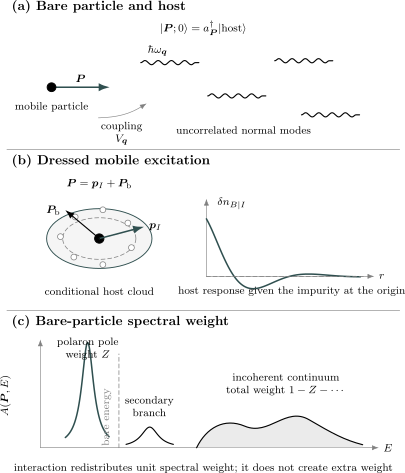
Three complementary views of polaron formation. A microscopic particle couples to host excitations and shares its conserved total momentum with them. The dressed state is diagnosed by conditional host correlations, not by a localized one-point density. In the bare-particle spectral function, interaction transfers weight from a bare line into a coherent polaron pole of residue $Z$, possible secondary branches, and an incoherent continuum.

Electron–Phonon Polarons

Physical origin

An electron changes the force experienced by nearby ions or polarizes an ionic crystal. The lattice responds, and that response acts back on the electron. Quantizing the lattice displacement converts the coupled problem into electron–phonon interactions.

The resulting polaron is not an electron plus a fixed number of phonons. Even in the ground state, virtual phonon configurations contribute coherently. Real phonon emission appears only when kinematics or temperature permits it.

Two minimal models emphasize different physics:

• the continuum Fröhlich model describes long-range coupling to polar optical modes;
• the lattice Holstein model describes local coupling between carrier density and an Einstein oscillator.

They should not be treated as interchangeable parameterizations.

Fröhlich continuum model

For one carrier in a polar crystal,

$$\begin{aligned} H_{\mathrm F} ={}& \frac{\hat{\mathbf P}^{\,2}}{2m_b} + \sum_{\mathbf q} \hbar\omega_{\mathrm{LO}} b_{\mathbf q}^\dagger b_{\mathbf q} \\ &+ \sum_{\mathbf q} \left( V_{\mathbf q} e^{i\mathbf q\cdot\hat{\mathbf R}} b_{\mathbf q} +\mathrm{h.c.} \right), \end{aligned}$$

where the idealized longitudinal-optical mode is dispersionless and

$$|V_{\mathbf q}|\propto\frac1q$$

in three dimensions, up to normalization and dielectric factors.

A conventional dimensionless coupling is

$$\alpha = \frac{e^2}{4\pi\epsilon_0\hbar} \sqrt{ \frac{m_b}{2\hbar\omega_{\mathrm{LO}}} } \left( \frac1{\epsilon_\infty} - \frac1{\epsilon_s} \right),$$

where $\epsilon_s$ and $\epsilon_\infty$ are relative static and high-frequency dielectric constants. A larger separation between ionic and electronic screening gives stronger lattice-polarization coupling.

At weak coupling,

$$E_0 = -\alpha\hbar\omega_{\mathrm{LO}} +O(\alpha^2),$$

and

$$\frac{m^*}{m_b} = 1+\frac\alpha6+O(\alpha^2).$$

These coefficients belong to the three-dimensional continuum Fröhlich convention. They are not generic weak-coupling coefficients for arbitrary phonon spectra.

Holstein lattice model

A minimal spinless one-carrier Holstein Hamiltonian is

$$\begin{aligned} H_{\mathrm H} ={}& -t\sum_{\langle ij\rangle} \left(c_i^\dagger c_j+\mathrm{h.c.}\right) \\ &+ \hbar\omega_0 \sum_i b_i^\dagger b_i \\ &+ g\sum_i n_i \left(b_i+b_i^\dagger\right). \end{aligned}$$

Here $g$ has units of energy. In the atomic limit $t=0$, occupying a site displaces its oscillator and lowers the energy by

$$E_p = \frac{g^2}{\hbar\omega_0}.$$

A local displacement transformation dresses hopping by oscillator translation operators. In a strong-coupling, low-temperature, antiadiabatic estimate,

$$t_{\mathrm{eff}} \sim t\exp\!\left[ -\left( \frac{g}{\hbar\omega_0} \right)^2 \right].$$

The exponentially narrowed band illustrates how a mobile carrier can become heavy. The estimate is not a universal equality: finite phonon frequency, dimensionality, longer-range hopping, multiple modes, and intermediate coupling modify it.

Large and small are physical regimes

A large polaron has a distortion spread over many lattice spacings, often making continuum intuition useful. A small polaron has strong local lattice correlation on the scale of one or a few unit cells and can exhibit strongly narrowed coherent hopping.

These labels concern cloud extent relative to the lattice, not merely whether $\alpha$ or $g$ is numerically large. A smooth crossover is common for one particle in a translation-invariant model. A variational state that localizes the carrier is not by itself proof of a thermodynamic symmetry-breaking transition.

Fermi Polarons

Mobile impurity in a Fermi sea

A Fermi polaron is a mobile impurity dressed primarily by particle–hole excitations of a Fermi sea. Let $c_{\mathbf k}$ annihilate a majority fermion and $d_{\mathbf K}$ annihilate the impurity. Here $\mathbf k$ and $\mathbf K$ are wave vectors, so the physical momenta are $\hbar\mathbf k$ and $\hbar\mathbf K$.

For a short-range interaction,

$$\begin{aligned} H={}& \sum_{\mathbf k} \epsilon_{\mathbf k\uparrow} c_{\mathbf k}^\dagger c_{\mathbf k} + \sum_{\mathbf K} \epsilon_{\mathbf K\downarrow} d_{\mathbf K}^\dagger d_{\mathbf K} \\ &+ \frac{g_0}{\mathcal V} \sum_{\mathbf k,\mathbf K,\mathbf q} c_{\mathbf k+\mathbf q}^\dagger d_{\mathbf K-\mathbf q}^\dagger d_{\mathbf K} c_{\mathbf k}. \end{aligned}$$

For continuum dispersions,

$$\epsilon_{\mathbf k\sigma} = \frac{\hbar^2k^2}{2m_\sigma}.$$

The bare contact coupling is cutoff-dependent. In three dimensions it can be related to the impurity–majority scattering length $a$ through

$$\frac1{g_0} = \frac{\mu_r}{2\pi\hbar^2a} - \frac1{\mathcal V} \sum_{\mathbf k} \frac{2\mu_r}{\hbar^2k^2},$$

where

$$\mu_r = \frac{m_\uparrow m_\downarrow} {m_\uparrow+m_\downarrow}$$

is the reduced mass. Observables depend on the renormalized scattering parameters rather than on $g_0$ separately.

At low impurity concentration, natural dimensionless controls include

$$\frac1{k_Fa}, \qquad \frac{m_\downarrow}{m_\uparrow}, \qquad \frac{T}{T_F},$$

plus effective range and dimensionality when relevant.

One particle–hole variational state

For total wave vector $\mathbf K$, the Chevy ansatz retains at most one majority particle–hole pair:

$$\begin{aligned} |\Psi_{\mathbf K}\rangle ={}& \alpha_0 d_{\mathbf K}^\dagger |\mathrm{FS}\rangle \\ &+ \sum_{\substack{q<k_F\\k>k_F}} \alpha_{\mathbf k\mathbf q} d_{\mathbf K+\mathbf q-\mathbf k}^\dagger c_{\mathbf k}^\dagger c_{\mathbf q} |\mathrm{FS}\rangle. \end{aligned}$$

Every term has the same particle numbers and the same total physical momentum $\hbar\mathbf K$. The ansatz makes the dressing cloud explicit as a coherent superposition of particle–hole pairs.

Its bare-component weight is

$$Z_{\mathbf K}=|\alpha_0|^2$$

after normalization within the ansatz. The variational equations resum repeated impurity–majority scattering in a restricted Hilbert space.

The one-pair approximation is often remarkably accurate for the three-dimensional attractive Fermi polaron, including near unitarity. That empirical success does not make it a systematic expansion in an obvious small parameter. More particle–hole sectors and independent methods remain essential benchmarks.

Attractive, repulsive, and molecular branches

For attractive interactions, the low-energy pole is called the attractive polaron. On the positive-scattering-length side, a bound impurity–majority dimer also exists in vacuum and can be dressed by the Fermi sea. Competition between polaron-like and molecule-like states is therefore natural.

A repulsive polaron can appear as a metastable excited branch associated with the upper scattering branch. It may be spectroscopically sharp over part of parameter space even though a lower-energy attractive state is available. Its lifetime is limited by decay into lower branches and continua.

The branch labels should not be reduced to the sign of a mean-field shift. A reliable identification uses

• the energy relative to the noninteracting impurity;
• spectral residue in the chosen probe;
• linewidth and decay channels;
• continuity under interaction tuning;
• pair correlations and molecular overlap;
• comparison with continuum thresholds.

There is no universal numerical polaron–molecule transition point independent of mass ratio, dimensionality, effective range, temperature, and approximation.

Bose Polarons

Microscopic impurity–boson model

Consider one impurity in an interacting Bose gas:

$$\begin{aligned} H={}& \frac{\hat{\mathbf P}^{\,2}}{2M} + \int d^dr\, \psi_B^\dagger \left( -\frac{\hbar^2\nabla^2}{2m_B} \right) \psi_B \\ &+ \frac{g_{BB}}2 \int d^dr\, \psi_B^\dagger\psi_B^\dagger \psi_B\psi_B \\ &+ g_{IB} \psi_B^\dagger(\hat{\mathbf R}) \psi_B(\hat{\mathbf R}). \end{aligned}$$

The last term couples the impurity to the local boson density. As with the Fermi contact model, bare zero-range couplings require ultraviolet renormalization in dimensions where the contact theory is singular.

Bogoliubov reduction

For a weakly depleted homogeneous condensate, write

$$\psi_B(\mathbf r) = \sqrt{n_0}+\delta\psi_B(\mathbf r).$$

Bogoliubov theory diagonalizes the quadratic host fluctuations. With

$$\epsilon_{\mathbf q}^{B} = \frac{\hbar^2q^2}{2m_B},$$

their dispersion is

$$E_{\mathbf q}^{B} = \sqrt{ \epsilon_{\mathbf q}^{B} \left( \epsilon_{\mathbf q}^{B}+2g_{BB}n_0 \right) }.$$

To linear order in host fluctuations, the impurity model becomes

$$\begin{aligned} H_{\mathrm{lin}} ={}& \frac{\hat{\mathbf P}^{\,2}}{2M} +g_{IB}n_0 + \sum_{\mathbf q} E_{\mathbf q}^{B} b_{\mathbf q}^\dagger b_{\mathbf q} \\ &+ \sum_{\mathbf q} \left( V_{\mathbf q}^{B} e^{i\mathbf q\cdot\hat{\mathbf R}} b_{\mathbf q} +\mathrm{h.c.} \right). \end{aligned}$$

For box-normalized modes,

$$V_{\mathbf q}^{B} = g_{IB} \sqrt{\frac{n_0}{\mathcal V}} \left(u_{\mathbf q}+v_{\mathbf q}\right),$$

with a phase convention in which

$$u_{\mathbf q}+v_{\mathbf q} = \sqrt{ \frac{\epsilon_{\mathbf q}^{B}} {E_{\mathbf q}^{B}} }.$$

The Bose polaron has therefore reduced to the generic bosonic model plus a mean-field shift $g_{IB}n_0$.

At small $q$,

$$E_{\mathbf q}^{B} \simeq \hbar cq,$$

and the density-coupling vertex is suppressed as

$$V_{\mathbf q}^{B}\propto\sqrt q.$$

This infrared structure reflects the rigidity of a compressible superfluid and strongly influences cloud and lifetime integrals.

Beyond the linear Fröhlich reduction

Expanding the impurity density coupling also produces terms quadratic in host fluctuations:

$$H = H_{\mathrm{lin}} +H_{2\mathrm{ph}} +\cdots.$$

The two-quasiparticle term contributes scattering of an existing host excitation and pair creation or annihilation. It can be important

• near an impurity–boson resonance;
• when condensate depletion is not weak;
• for short-distance pair correlations;
• when bound clusters or three-body processes matter;
• when ultraviolet renormalization is treated quantitatively.

The linear Fröhlich form is therefore a controlled low-fluctuation reduction only within an identified regime. It is not a universal strong-coupling Bose-polaron Hamiltonian.

Fermi and Bose environments differ

Feature	Fermi polaron	Bose polaron
dominant weak excitations	particle–hole pairs	Bogoliubov modes
infrared host scale	Fermi surface and $v_F$	sound velocity and healing length
simple variational language	Chevy particle–hole expansion	coherent or correlated phonon state
nearby bound structures	dressed dimer and holes	impurity–boson clusters and medium dressing
statistics constraint	Pauli blocking	Bose enhancement and condensate coherence

Both are mobile-impurity problems, but their infrared phase space and strong-coupling few-body physics are qualitatively different.

A Unified View of Branches

Ground-state branch

At fixed total momentum, the lowest state in the impurity sector defines the ground-state dispersion when it remains identifiable in the thermodynamic limit. It can evolve from weakly dressed particle-like behavior toward a strongly correlated or molecule-like state.

Calling the lowest state a polaron is most informative when

• it has a coherent mobile branch;
• it is continuously connected to a bare impurity or carrier in a useful parameter regime;
• its observables are captured by dressed-particle variables;
• it is separated enough from continua for energy and curvature to be meaningful.

Metastable branch

An excited pole can be useful even when it is not the lowest state. It must have a lifetime long compared with the measurement or dynamical timescale:

$$\Gamma_E \ll \Delta E_{\mathrm{resolve}},$$

where $\Delta E_{\mathrm{resolve}}$ is the separation from nearby structures or the relevant experimental energy scale.

“Repulsive polaron” and similar labels usually describe such metastable branches. Their existence is scale-dependent, not absolute.

Molecular and continuum sectors

A molecule-like state contains a strong bound pair or cluster dressed by the medium. It may have nonzero overlap with a bare impurity operator because interactions mix sectors visible to the probe. Conversely, a continuum can carry substantial spectral weight without defining one particle-like branch.

Avoid the false dichotomy

$$\text{polaron} \quad\text{or}\quad \text{molecule}.$$

At finite volume, exact eigenstates mix all configurations allowed by symmetry. The useful question is which effective description organizes the low-energy spectrum and observables in the regime of interest.

Approximation Strategies

Weak-coupling perturbation theory

Expanding in $V_{\mathbf q}$ gives transparent formulas for energy, mass, residue, and emission rates. It is controlled when all relevant dimensionless corrections are small and no infrared or ultraviolet divergence invalidates termwise expansion.

Strengths include

• analytic limiting behavior;
• direct recoil interpretation;
• exact checks on signs and dimensions;
• systematic order counting when the series is controlled.

Limitations include

• poor description of bound states or large clouds;
• secular or singular behavior near thresholds;
• dependence on proper coupling renormalization.

Perturbation Theory in Many-Body Systems owns the general linked-diagram and order-counting framework.

Coherent-state and Lee–Low–Pines variational methods

A simple LLP-frame ansatz is

$$|\Phi_{\mathbf P}\rangle = \exp\!\left[ \sum_{\mathbf q} \left( \alpha_{\mathbf q}b_{\mathbf q}^\dagger -\alpha_{\mathbf q}^*b_{\mathbf q} \right) \right] |0\rangle.$$

Minimizing

$$E_{\mathrm{var}}(\mathbf P) = \frac{ \langle\Phi_{\mathbf P}| \widetilde H_{\mathbf P} |\Phi_{\mathbf P}\rangle }{ \langle\Phi_{\mathbf P}|\Phi_{\mathbf P}\rangle }$$

allows a many-boson cloud at modest cost. Correlated Gaussian states, squeezed states, and non-Gaussian extensions can capture mode–mode recoil correlations missed by a product coherent state.

The variational energy is an upper bound for a Hermitian Hamiltonian in the stated sector. Residue, cloud shape, and dynamics are not automatically bounded with the same reliability.

Feynman path-integral method

For the Fröhlich polaron, integrating out harmonic phonons produces a retarded self-interaction along the carrier path. Feynman’s quadratic trial action gives an influential variational interpolation between weak and strong coupling.

Its conceptual lesson is broader than one formula: eliminating a Gaussian environment trades explicit bosons for nonlocality in imaginary time. An apparently one-particle action can therefore retain many-body memory.

Ladder and T-matrix methods

For resonant short-range impurity problems, repeated two-body scattering is essential. A medium T-matrix resums ladder diagrams and enters the impurity self-energy.

This captures scattering-length renormalization, Pauli blocking in a Fermi sea, and medium-shifted pair propagation. Its accuracy depends on whether omitted vertex corrections, multiple particle–hole sectors, condensate fluctuations, or three-body correlations are important.

Diagrammatic Methods Preview owns the general diagram grammar and consistency requirements.

Numerical methods

Useful nonperturbative tools include

• diagrammatic Monte Carlo for continuum polarons;
• diffusion or auxiliary-field Monte Carlo when signs and trial-state bias are controlled;
• exact diagonalization for truncated momentum or lattice Hilbert spaces;
• density-matrix renormalization and tensor networks in one dimension;
• variational Monte Carlo with explicitly correlated states;
• real-time methods for formation and spectroscopy.

Every numerical result should report cutoff, volume, basis, time window, statistical error, and extrapolation strategy. Agreement of energy alone does not validate residue, linewidth, and cloud correlations.

Controlled Limits and Cross-Checks

Zero coupling

As the interaction vanishes,

$$V_{\mathbf q}\to0,$$

a particle-like polaron branch should satisfy

$$E(\mathbf P)\to\epsilon_{\mathbf P}, \qquad Z_{\mathbf P}\to1, \qquad M^*\to M.$$

Failure indicates a convention, normalization, branch-tracking, or extrapolation problem.

Infinite mass

As $M\to\infty$, recoil disappears and the linear boson model reduces to independent displaced oscillators. Any proposed method for that model should reproduce

$$\Delta E_\infty = -\sum_{\mathbf q} \frac{|V_{\mathbf q}|^2} {\hbar\omega_{\mathbf q}}.$$

This is a stringent test because it probes all boson numbers, not merely second order.

High momentum

At large total momentum, the low-energy branch may intersect emission continua. A real variational dispersion without a corresponding width can then be misleading. One should compare

$$E(\mathbf P)$$

against all accessible thresholds and inspect the spectral function rather than extrapolating the small-$P$ effective mass.

Sum rules

For a canonical bare impurity operator in the single-particle spectral convention,

$$\int_{-\infty}^{\infty} dE\, A(\mathbf P,E)=1.$$

If a pole carries weight $Z_{\mathbf P}$, the remaining weight belongs to other poles and continua:

$$Z_{\mathbf P} + \int_{\mathrm{inc}} dE\, A(\mathbf P,E) =1.$$

A truncated calculation that reports a residue but violates the total sum rule has not consistently accounted for omitted states.

Hellmann–Feynman diagnostics

If a Hamiltonian depends on coupling $\lambda$ and the state is a differentiable exact eigenstate,

$$\frac{\partial E}{\partial\lambda} = \left\langle \frac{\partial H}{\partial\lambda} \right\rangle.$$

This can connect derivatives of the polaron energy to interaction expectation values or contacts. Such derivatives often provide more robust checks than inferring cloud composition from a schematic wavefunction.

Polaron Formation Is Dynamical

Sudden injection

Spectroscopy often creates a bare impurity or transfers an atom into an interacting internal state suddenly. The initial state is then a superposition of polaron poles and continua:

$$|\Psi(0)\rangle = \sqrt Z\,|\mathrm{pol}\rangle + \sum_n c_n|n,\mathrm{inc}\rangle.$$

Its return amplitude contains

$$\mathcal S(t) = \langle\Psi(0)|e^{-iHt/\hbar}|\Psi(0)\rangle.$$

A stable pole contributes a persistent oscillatory term of magnitude $Z$, while a continuum dephases. A metastable pole contributes an exponentially damped component only over the time window where a simple pole approximation is valid.

Dressing time

There is no single universal cloud-formation time. Candidate scales include

$$\begin{gathered} \omega_{\mathrm{host}}^{-1}, \qquad \dfrac{\hbar}{|E_0-E_{\mathrm{bare}}|} \\ \dfrac{R_{\mathrm{cloud}}}{c}, \qquad \tau_{\mathrm{decay}}. \end{gathered}$$

Different observables can equilibrate on different scales. Short-range pair correlations may build before a long-wavelength density disturbance has propagated across the cloud.

Adiabatic preparation

Slowly ramping the interaction can prepare a ground-state polaron only when the ramp is slow relative to relevant gaps and no thermodynamic continuum destroys adiabaticity. In a gapless host, arbitrarily low-energy excitations make the strict infinite-system adiabatic limit delicate.

Finite size, finite temperature, finite duration, and observable resolution must therefore be part of any preparation claim.

Breakdown of the Polaron Picture

Vanishing residue

If

$$Z_{\mathbf P}\to0$$

in the thermodynamic limit, the bare particle operator does not create a finite-weight pole. The spectrum may instead show a threshold singularity or broad continuum. This can arise through infrared orthogonality even when the energy remains finite.

The absence of residue is operator-specific, but it is a decisive failure of the corresponding bare-particle quasiparticle picture.

Strong binding and clusters

Near resonance, an impurity may bind one or more host particles. Then a molecular or cluster degree of freedom can organize the spectrum better than a dressed elementary impurity. Three-body parameters and losses may become essential, especially in Bose gases.

Finite impurity density

The one-polaron limit neglects impurity–impurity overlap and induced interactions. At finite density, dressing clouds can mediate interactions, Pauli statistics can matter for fermionic impurities, and a coherent polaron gas may undergo pairing, phase separation, or other collective phenomena.

One-polaron parameters can seed an effective theory, but they do not determine it completely.

Disorder and localization

Disorder breaks momentum conservation and can localize the impurity or host modes. The Lee–Low–Pines momentum-sector construction then no longer applies globally. Effective mass may cease to be the useful transport variable even if local dressing remains strong.

No sharp separation of particle and cloud

The division into bare particle and environment depends on the microscopic basis and canonical transformation. Physical predictions are invariant, but quantities such as phonon number can change under a unitary redefinition of modes.

Energy differences, response functions, conserved charges, and specified correlation functions are more robust than an unqualified statement that the polaron contains a particular number of phonons.

Experimental Diagnostics

Radio-frequency and Raman spectroscopy

In ultracold gases, an internal-state transfer can inject an impurity into an interacting channel. The transfer rate probes a convolution of initial occupation, final-state spectral weight, matrix elements, and pulse shape.

A coherent polaron can produce a peak whose

• position estimates an interaction energy;
• integrated weight can constrain $Z$ after calibration;
• width combines intrinsic decay, inhomogeneity, temperature, and instrumental broadening.

Peak area equals quasiparticle residue only under a derived spectroscopy protocol.

Momentum-resolved probes

Resolving transferred momentum maps a branch $E(\mathbf P)$ and allows a curvature mass to be fitted near its minimum. The fit window must remain below nonparabolic and decay-threshold scales.

Real-space correlations

Species-selective imaging or pair-correlation measurements can access the conditional cloud. A useful observable may be

$$g_{IB}^{(2)}(\mathbf r) = \frac{ \langle n_I(\mathbf0)n_B(\mathbf r)\rangle }{ \langle n_I(\mathbf0)\rangle \langle n_B(\mathbf r)\rangle }.$$

At short distance this can be sensitive to contact physics and resolution; at long distance it probes the host response and cloud extent.

Transport and optical response

In solids, conductivity, mobility, optical sidebands, photoemission, tunneling, isotope effects, and temperature dependence can all reveal electron–phonon dressing. None is a one-number measurement of the polaron. A material interpretation must distinguish band structure, disorder, multiple phonon branches, carrier density, screening, and vertex effects.

Worked Example: Recoil and Infrared Dressing

Consider an idealized acoustic bath in $d$ dimensions with

$$\omega_q=cq$$

and low-momentum coupling

$$|V_q|^2\propto q^s.$$

At finite impurity mass,

$$D_q = \hbar cq + \frac{\hbar^2q^2}{2M} \sim q$$

as $q\to0$. The weak-coupling energy integral scales as

$$\int_0 dq\, q^{d-1} \frac{q^s}{q} = \int_0 dq\, q^{d+s-2}.$$

It is infrared convergent when

$$d+s>1.$$

The residue correction scales as

$$\int_0 dq\, q^{d-1} \frac{q^s}{q^2} = \int_0 dq\, q^{d+s-3},$$

which converges only when

$$d+s>2.$$

There is therefore an intermediate range

$$1<d+s\le2$$

in which the energy is infrared finite but the perturbative residue is not. The exact infrared physics then requires resummation and may exhibit orthogonality rather than a finite pole.

Worked Example: Mean-Field Bose-Polaron Shift

For a uniform condensate and weak impurity–boson coupling, replace the host density at leading order by $n_0$. The interaction energy is

$$E_{\mathrm{MF}} = g_{IB}n_0.$$

In three dimensions, the low-energy coupling is

$$g_{IB} = \frac{2\pi\hbar^2a_{IB}}{\mu_r}$$

at leading pseudopotential order, where $a_{IB}$ is the impurity–boson scattering length and $\mu_r$ the reduced mass. Hence

$$E_{\mathrm{MF}} = \frac{2\pi\hbar^2a_{IB}n_0}{\mu_r}.$$

This is linear in density and scattering length. It does not include condensate deformation, phonon dressing, effective-range corrections, or bound-state physics. Near resonance, the expression is not a controlled energy formula.

Worked Example: Momentum Bookkeeping in a Fermi Cloud

Take one term of the Chevy ansatz,

$$d_{\mathbf K+\mathbf q-\mathbf k}^\dagger c_{\mathbf k}^\dagger c_{\mathbf q} |\mathrm{FS}\rangle.$$

Relative to the Fermi sea, its total wave vector is

$$(\mathbf K+\mathbf q-\mathbf k) +\mathbf k-\mathbf q = \mathbf K.$$

The particle–hole excitation carries $\mathbf k-\mathbf q$, while the impurity carries the compensating wave vector $\mathbf K+\mathbf q-\mathbf k$. The cloud and impurity momenta fluctuate separately, but their sum is fixed in every basis component.

Common Mistakes

• Treating the cloud as a static object in the laboratory frame. A momentum eigenstate is translation invariant; use conditional correlations.
• Calling every shifted impurity line a polaron. A useful quasiparticle requires a trackable pole or branch with a stated lifetime and overlap.
• Equating residue with one minus boson number. That relation holds only perturbatively or in special coherent-state models.
• Dropping recoil without stating an infinite-mass approximation. Recoil changes energies, masses, thresholds, and mode correlations.
• Using a bare contact coupling as an observable. Zero-range models require regularization and matching to scattering parameters.
• Reading effective mass as drag or mobility. Mass is dispersion curvature; transport also requires momentum relaxation.
• Assuming a real variational energy implies stability. Compare the branch with every allowed continuum and compute a width when decay is open.
• Calling a metastable repulsive branch a ground state. Branch energy ordering and lifetime must both be stated.
• Using the Fröhlich reduction near resonance without two-phonon terms. The linear model can miss short-distance and few-body physics.
• Interpreting a self-localized variational wavefunction as automatic symmetry breaking. Restore translation symmetry and compare exact finite-system quantum numbers.
• Quoting a universal polaron–molecule transition number. It depends on masses, dimension, range, temperature, and model.
• Fitting a mass too far from the branch minimum. Higher-order dispersion and emission thresholds can dominate.
• Ignoring spectral sum rules. Pole weight removed from one feature must reappear elsewhere.
• Confusing localized Anderson impurities with mobile polarons. Hybridization of a fixed orbital and recoil of a moving impurity are different organizing problems.

Decision Checklist

Before calling an excitation a polaron, ask:

1. What microscopic operator creates the bare particle?
2. Which environmental excitations dress it?
3. What is the conserved total momentum or lattice crystal momentum?
4. Is the observed feature a pole, a resonance, a threshold, or a broad continuum?
5. How are $E$, $M^*$, $Z$, and $\Gamma_E$ defined and extracted?
6. Which conditional correlation defines the cloud?
7. Are ultraviolet couplings properly renormalized?
8. Which decay channels are kinematically open?
9. What small parameter or variational principle controls the approximation?
10. Do zero-coupling, infinite-mass, sum-rule, and finite-size checks pass?
11. Is a competing molecule or cluster a better low-energy variable?
12. Does the one-impurity limit apply at the stated concentration?

Exercises

Exercise 1: Total momentum conservation

For the generic mobile-impurity Hamiltonian, show directly that

$$[H,\hat{\mathbf P}_{\mathrm{tot}}]=0.$$

Track the impurity and boson momentum changes in one interaction term.

Solution

The free impurity and free-boson Hamiltonians commute with their own momenta and with the other subsystem’s momentum. It remains to test

$$X_{\mathbf q} = e^{i\mathbf q\cdot\hat{\mathbf R}} b_{\mathbf q}.$$

Using

$$[\hat{\mathbf P}, e^{i\mathbf q\cdot\hat{\mathbf R}}] = \hbar\mathbf q\, e^{i\mathbf q\cdot\hat{\mathbf R}}$$

and

$$[\hat{\mathbf P}_{\mathrm b},b_{\mathbf q}] = -\hbar\mathbf q\,b_{\mathbf q},$$

we find

$$[\hat{\mathbf P},X_{\mathbf q}] = \hbar\mathbf q\,X_{\mathbf q},$$

while

$$[\hat{\mathbf P}_{\mathrm b},X_{\mathbf q}] = -\hbar\mathbf q\,X_{\mathbf q}.$$

The terms cancel, so

$$[\hat{\mathbf P}_{\mathrm{tot}},X_{\mathbf q}]=0.$$

The Hermitian-conjugate interaction also commutes. Therefore the complete Hamiltonian conserves total momentum. Annihilating a boson transfers $+\hbar\mathbf q$ to the impurity; creating one transfers $-\hbar\mathbf q$.

Exercise 2: Lee–Low–Pines transformation

Starting from

$$\mathcal U_{\mathrm{LLP}} = \exp\!\left( -\frac{i}{\hbar} \hat{\mathbf R}\cdot\hat{\mathbf P}_{\mathrm b} \right),$$

derive the transformed Hamiltonian in a sector of total momentum $\mathbf P$.

Solution

The Baker–Campbell–Hausdorff expansion terminates for the impurity momentum because $\hat{\mathbf P}_{\mathrm b}$ commutes with $\hat{\mathbf R}$:

$$\mathcal U_{\mathrm{LLP}}^\dagger \hat{\mathbf P} \mathcal U_{\mathrm{LLP}} = \hat{\mathbf P}-\hat{\mathbf P}_{\mathrm b}.$$

For a boson operator, the nested commutators exponentiate:

$$\mathcal U_{\mathrm{LLP}}^\dagger b_{\mathbf q} \mathcal U_{\mathrm{LLP}} = e^{-i\mathbf q\cdot\hat{\mathbf R}} b_{\mathbf q}.$$

Hence the position factors in the interaction cancel. The transformed total momentum is $\hat{\mathbf P}$, so in its eigen-sector one replaces that operator by the conserved value $\mathbf P$. The result is

$$\begin{aligned} \widetilde H_{\mathbf P} ={}& \frac{ (\mathbf P-\hat{\mathbf P}_{\mathrm b})^2 }{2M} + \sum_{\mathbf q} \hbar\omega_{\mathbf q}n_{\mathbf q} \\ &+ \sum_{\mathbf q} \left( V_{\mathbf q}b_{\mathbf q} +V_{\mathbf q}^*b_{\mathbf q}^\dagger \right). \end{aligned}$$

The impurity coordinate is absent, while recoil generates interactions among boson occupations through $\hat{\mathbf P}_{\mathrm b}^{\,2}$.

Exercise 3: Static cloud and overlap

For the static-impurity Hamiltonian, derive the ground-state energy shift, mean boson number, and bare-vacuum residue.

Solution

Complete the square mode by mode with

$$c_{\mathbf q} = b_{\mathbf q} + \frac{V_{\mathbf q}^*} {\hbar\omega_{\mathbf q}}.$$

Then

$$H_\infty = \sum_{\mathbf q} \hbar\omega_{\mathbf q} c_{\mathbf q}^\dagger c_{\mathbf q} - \sum_{\mathbf q} \frac{|V_{\mathbf q}|^2} {\hbar\omega_{\mathbf q}}.$$

The $c$-vacuum is a product of $b$-coherent states with

$$\alpha_{\mathbf q} = -\frac{V_{\mathbf q}^*} {\hbar\omega_{\mathbf q}}.$$

Therefore

$$\Delta E_\infty = -\sum_{\mathbf q} \frac{|V_{\mathbf q}|^2} {\hbar\omega_{\mathbf q}},$$ $$N_{\mathrm b} = \sum_{\mathbf q} \frac{|V_{\mathbf q}|^2} {(\hbar\omega_{\mathbf q})^2},$$

and the product coherent-state overlap gives

$$Z_\infty = \exp(-N_{\mathrm b}).$$

The last identity uses the coherent-product structure and should not be exported unchanged to generic interacting polarons.

Exercise 4: Weak-coupling mass enhancement

Expand the second-order energy $E(\mathbf P)$ through $P^2$ for an isotropic bath and show that the correction increases the mass.

Solution

Write

$$x_{\mathbf q} = \frac{\mathbf P\cdot\hbar\mathbf q}{M}.$$

Then

$$\frac1{D_{\mathbf q}-x_{\mathbf q}} = \frac1{D_{\mathbf q}} + \frac{x_{\mathbf q}}{D_{\mathbf q}^2} + \frac{x_{\mathbf q}^2}{D_{\mathbf q}^3} +O(P^3).$$

Inversion symmetry removes the linear term. Isotropy gives

$$\sum_{\mathbf q} q_iq_jF(q) = \frac{\delta_{ij}}d \sum_{\mathbf q}q^2F(q).$$

Therefore

$$\frac1{2M^*} = \frac1{2M} - \frac1{dM^2} \sum_{\mathbf q} \frac{ |V_{\mathbf q}|^2\hbar^2q^2 }{D_{\mathbf q}^3}.$$

Every term in the correction is nonnegative, so the inverse mass decreases. Within the perturbative regime,

$$M^*>M.$$

If the correction becomes comparable to $1/M$, the expansion has left its domain and cannot establish an infinite or negative mass.

Exercise 5: Emission threshold

For a parabolic polaron branch

$$E(\mathbf P)=E_0+\frac{P^2}{2M^*}$$

and an acoustic host mode $\omega_q=cq$, determine the small-$q$ threshold for one-mode emission.

Solution

Energy conservation requires

$$\frac{P^2}{2M^*} \ge \frac{|\mathbf P-\hbar\mathbf q|^2}{2M^*} + \hbar cq.$$

After cancellation,

$$\frac{\mathbf P\cdot\mathbf q}{M^*} - \frac{\hbar q^2}{2M^*} \ge cq.$$

For $q\to0$, the most favorable emission is parallel to $\mathbf P$, yielding

$$\frac{P}{M^*}\ge c.$$

Thus the small-$q$ threshold is reached when the polaron group velocity equals the sound velocity. At finite $q$, recoil adds the positive requirement $\hbar q/(2M^*)$, and the exact threshold must minimize over the full dispersions.

Exercise 6: Chevy-state bookkeeping

Verify that every term in the one-particle–hole Chevy ansatz has the same majority number, impurity number, and total momentum.

Solution

The bare term adds one impurity and leaves the majority Fermi sea unchanged. A dressed term contains

$$c_{\mathbf k}^\dagger c_{\mathbf q},$$

which removes one occupied majority state $\mathbf q$ and fills one unoccupied state $\mathbf k$. The majority particle number is unchanged, and $d^\dagger$ adds exactly one impurity.

The total wave vector relative to the Fermi sea is

$$(\mathbf K+\mathbf q-\mathbf k) +(\mathbf k-\mathbf q) = \mathbf K.$$

Thus all components lie in the same conserved sector. This bookkeeping is why the impurity momentum in the dressed term cannot remain $\mathbf K$.

Exercise 7: Three cloud diagnostics

Explain why the following need not be equal:

$$\begin{gathered} 1-Z, \\ \displaystyle \sum_{\mathbf q} \langle b_{\mathbf q}^\dagger b_{\mathbf q}\rangle, \\ \displaystyle \int d^dr\, \delta n_{B|I}(\mathbf r). \end{gathered}$$

Give one limit in which a relation between the first two does hold.

Solution

$1-Z$ is loss of overlap with a specified bare insertion state. The boson sum counts excitations in a chosen quasiboson basis. The density integral counts net host-particle excess or depletion conditioned on the impurity. A Bogoliubov quasiboson is a particle–hole mixture of host modes, so its number is not a host-particle number. Moreover, different many-boson configurations can be orthogonal to the bare state without carrying a net density excess.

For the exact static linear-boson model, the ground state is a product coherent state and

$$Z=e^{-N_{\mathrm b}},$$

where

$$N_{\mathrm b} = \sum_{\mathbf q} \langle b_{\mathbf q}^\dagger b_{\mathbf q}\rangle.$$

At weak coupling this gives

$$1-Z=N_{\mathrm b}+O(V^4).$$

Neither relation determines the integrated conditional density in a generic host.

Exercise 8: Bose-polaron linear vertex

Starting from

$$g_{IB}\psi_B^\dagger(\hat{\mathbf R}) \psi_B(\hat{\mathbf R}),$$

expand around a uniform condensate and recover the mean-field shift and linear Bogoliubov coupling.

Solution

Write

$$\psi_B(\mathbf r) = \sqrt{n_0}+\delta\psi_B(\mathbf r).$$

Then

$$\begin{aligned} \psi_B^\dagger\psi_B ={}& n_0 + \sqrt{n_0} \left( \delta\psi_B+\delta\psi_B^\dagger \right) \\ &+ \delta\psi_B^\dagger\delta\psi_B. \end{aligned}$$

The first term gives $g_{IB}n_0$. Expand the fluctuation field in box-normalized Bogoliubov modes. In a convention with

$$\begin{aligned} \delta\psi_B+\delta\psi_B^\dagger ={}& \frac1{\sqrt{\mathcal V}} \sum_{\mathbf q} (u_{\mathbf q}+v_{\mathbf q}) \\ &\times \left( e^{i\mathbf q\cdot\mathbf r}b_{\mathbf q} + e^{-i\mathbf q\cdot\mathbf r}b_{\mathbf q}^\dagger \right), \end{aligned}$$

the linear interaction at $\mathbf r=\hat{\mathbf R}$ is

$$\sum_{\mathbf q} \left( V_{\mathbf q}^{B} e^{i\mathbf q\cdot\hat{\mathbf R}} b_{\mathbf q} +\mathrm{h.c.} \right),$$

with

$$V_{\mathbf q}^{B} = g_{IB} \sqrt{\frac{n_0}{\mathcal V}} (u_{\mathbf q}+v_{\mathbf q}).$$

The quadratic fluctuation term becomes $H_{2\mathrm{ph}}$ and is omitted only in the linear Fröhlich reduction.

Summary

• A polaron is a mobile particle and its correlated environmental response treated as one dressed excitation.
• Total momentum belongs to the combined particle–host system; recoil is central at finite impurity mass.
• The Lee–Low–Pines transformation removes the impurity coordinate exactly and exposes momentum sharing and recoil-induced mode coupling.
• The infinite-mass linear-boson model is an exact product of displaced oscillators, with a negative dressing energy and residue $Z=e^{-N_{\mathrm b}}$.
• Weak coupling lowers the energy, reduces bare-particle residue, and usually increases the isotropic effective mass.
• Energy, mass, residue, linewidth, boson number, and conditional cloud density are distinct observables.
• A sharp pole can be stable or metastable; emission begins when a lower branch plus host excitation satisfies energy and momentum conservation.
• Fröhlich and Holstein models capture different electron–phonon regimes.
• Fermi polarons are dressed by particle–hole excitations; Bose polarons are dressed by condensate collective modes and can require beyond-Fröhlich terms near resonance.
• Molecular branches, infrared orthogonality, strong binding, finite density, disorder, and open decay channels can invalidate a simple finite-residue polaron description.

References

1. T. D. Lee, F. E. Low, and D. Pines, “The motion of slow electrons in a polar crystal,” Physical Review 90, 297–302 (1953), doi:10.1103/PhysRev.90.297. Canonical transformation and translationally invariant treatment of the Fröhlich polaron.
2. H. Fröhlich, “Electrons in lattice fields,” Advances in Physics 3, 325–361 (1954), doi:10.1080/00018735400101213. Continuum coupling of a carrier to polar optical modes.
3. R. P. Feynman, “Slow electrons in a polar crystal,” Physical Review 97, 660–665 (1955), doi:10.1103/PhysRev.97.660. Path-integral variational treatment across coupling regimes.
4. T. Holstein, “Studies of polaron motion: Part I. The molecular-crystal model,” Annals of Physics 8, 325–342 (1959), doi:10.1016/0003-4916(59)90002-8. Local lattice polaron and hopping model.
5. J. T. Devreese and A. S. Alexandrov, “Fröhlich polaron and bipolaron: Recent developments,” Reports on Progress in Physics 72, 066501 (2009), doi:10.1088/0034-4885/72/6/066501. Broad review of continuum and lattice polaron physics.
6. F. Giustino, “Electron–phonon interactions from first principles,” Reviews of Modern Physics 89, 015003 (2017), doi:10.1103/RevModPhys.89.015003. Microscopic electron–phonon matrix elements and materials calculations.
7. F. Chevy, “Universal phase diagram of a strongly interacting Fermi gas with unbalanced spin populations,” Physical Review A 74, 063628 (2006), doi:10.1103/PhysRevA.74.063628. One-particle–hole variational construction.
8. R. Combescot, A. Recati, C. Lobo, and F. Chevy, “Normal state of highly polarized Fermi gases: Simple many-body approaches,” Physical Review Letters 98, 180402 (2007), doi:10.1103/PhysRevLett.98.180402. Fermi-polaron energy and variational/T-matrix comparison.
9. N. Prokof’ev and B. Svistunov, “Fermi-polaron problem: Diagrammatic Monte Carlo method for divergent sign-alternating series,” Physical Review B 77, 020408 (2008), doi:10.1103/PhysRevB.77.020408. Numerically exact diagrammatic benchmarking.
10. A. Schirotzek, C.-H. Wu, A. Sommer, and M. W. Zwierlein, “Observation of Fermi polarons in a tunable Fermi liquid of ultracold atoms,” Physical Review Letters 102, 230402 (2009), doi:10.1103/PhysRevLett.102.230402. Spectroscopic observation of Fermi-polaron energy and residue.
11. P. Massignan, M. Zaccanti, and G. M. Bruun, “Polarons, dressed molecules and itinerant ferromagnetism in ultracold Fermi gases,” Reports on Progress in Physics 77, 034401 (2014), doi:10.1088/0034-4885/77/3/034401. Review of Fermi-polaron branches, methods, and experiments.
12. F. Scazza, G. Valtolina, P. Massignan, A. Recati, A. Amico, A. Burchianti, C. Fort, M. Inguscio, M. Zaccanti, and G. Roati, “Repulsive Fermi polarons in a resonant mixture of ultracold lithium-6 atoms,” Physical Review Letters 118, 083602 (2017), doi:10.1103/PhysRevLett.118.083602. Metastable repulsive-branch spectroscopy and decay.
13. N. B. Jørgensen, L. Wacker, K. T. Skalmstang, M. M. Parish, J. Levinsen, R. S. Christensen, G. M. Bruun, and J. J. Arlt, “Observation of attractive and repulsive polarons in a Bose–Einstein condensate,” Physical Review Letters 117, 055302 (2016), doi:10.1103/PhysRevLett.117.055302. Bose-polaron spectroscopy across impurity–boson interaction strength.
14. M.-G. Hu, M. J. Van de Graaff, D. Kedar, J. P. Corson, E. A. Cornell, and D. S. Jin, “Bose polarons in the strongly interacting regime,” Physical Review Letters 117, 055301 (2016), doi:10.1103/PhysRevLett.117.055301. Experimental strong-coupling Bose-polaron response.
15. F. Grusdt, R. Schmidt, Y. E. Shchadilova, and E. Demler, “Strong-coupling Bose polarons in a Bose–Einstein condensate,” Physical Review A 96, 013607 (2017), doi:10.1103/PhysRevA.96.013607. Renormalization-group and variational analysis beyond elementary weak coupling.
16. C. Lobo, A. Recati, S. Giorgini, and S. Stringari, “Normal state of a polarized Fermi gas at unitarity,” Physical Review Letters 97, 200403 (2006), doi:10.1103/PhysRevLett.97.200403. Dilute-minority equation of state and quasiparticle interpretation.
17. G. D. Mahan, Many-Particle Physics, 3rd ed. (Springer, 2000), doi:10.1007/978-1-4757-5714-9. Green functions, electron–phonon coupling, canonical transformations, and spectral response.

Cross-Links

• Quasiparticles Overview
• Collective Modes
• Phonons as Many-Body Excitations
• Particle–Hole Excitations
• Spectral Functions
• Green Functions in Many-Body QM
• Bogoliubov Theory
• Weakly Interacting Bose Gas Preview
• Diagrammatic Methods Preview
• Effective Mass
• Condensed-Matter Roadmap