Particle–Hole Excitations

A particle–hole excitation is produced when a fermion is removed from an occupied one-particle mode and placed in an unoccupied mode. Relative to the chosen filled reference, the promoted fermion is the particle and the missing occupation is the hole. The pair preserves microscopic particle number but carries energy, momentum, spin, and other quantum numbers into the many-body system.

For a translation-invariant independent Fermi sea,

$$\lvert \mathbf k+\mathbf q,\alpha; \mathbf k,\beta^{-1} \rangle := c_{\mathbf k+\mathbf q,\alpha}^{\dagger} c_{\mathbf k,\beta} \lvert\mathrm{FS}\rangle.$$

This state is nonzero only when the initial mode is occupied and the final mode is empty. Its excitation energy is

$$\Delta\epsilon_{\mathbf k,\mathbf q}^{\alpha\beta} := \epsilon_{\mathbf k+\mathbf q,\alpha} - \epsilon_{\mathbf k,\beta},$$

and its total momentum transfer is $\hbar\mathbf q$, modulo a reciprocal-lattice vector when the system is crystalline.

One pair has a definite energy for fixed labels. A particle–hole continuum appears because many occupied initial modes can be promoted to many empty final modes with the same transferred momentum. In finite volume these are discrete lines. Their spacing becomes dense in the thermodynamic limit, and an experiment with finite resolution sees a continuous spectral region.

Scope and Canonical Ownership

This page owns the generic excitation concept:

• the filled reference sea and the conditions for a nonzero promotion;
• hole operators, positive hole energy, and the signs of hole momentum and charge;
• normalized one-pair states and their conserved quantum numbers;
• the difference between a hole label and the physical momentum of the missing particle;
• density, spin, current, and general one-body operators as creators of pair superpositions;
• the joint phase-space density that becomes the particle–hole continuum;
• continuum boundaries for an isotropic parabolic band;
• the special one-dimensional kinematics;
• the connection between continuum weight and the imaginary part of a response function;
• finite-temperature smearing, interactions, collective modes, and multi-pair states;
• distinctions from particle–hole symmetry, Bogoliubov mixing, excitons, and antiparticles.

Neighboring pages retain more specialized ownership:

• Holes owns the nearly-full crystalline-band specialization, exact state count per cell, crystal momentum modulo reciprocal vectors, group-current sign ledger, and degenerate or multiband valence-band limits.
• Fermi Surface owns the ground-state occupation boundary, Fermi-surface geometry, velocity, density of states, and low-energy shell.
• Ideal Fermi Gas owns equilibrium thermodynamics and the relation among density, Fermi momentum, and Fermi energy.
• Density Operators and Current Operators owns local conservation laws and operator conventions.
• Structure Factors owns static and dynamic normalization, detailed balance, sum rules, and scattering cross sections.
• Susceptibilities owns source conventions, units, response tensors, and orders of limits.
• Random Phase Approximation owns the Lindhard evaluation as an input to screening, bubble resummation, dielectric response, and collective poles.
• Quasiparticles Overview owns the general tests for particle-like poles, residues, lifetimes, and breakdown.
• Bogoliubov Quasiparticles owns coherent creation–annihilation mixing. An ordinary particle–hole pair instead has one creation operator and one annihilation operator and preserves microscopic number.
• Polarons Preview owns a mobile impurity dressed by a coherent superposition of these particle–hole excitations in a Fermi sea.

The purpose here is to make the excitation kinematics and response interpretation reusable without duplicating the full thermodynamics, response dictionary, or RPA calculation.

The Filled Reference Sea

Zero-temperature reference

Let

$$K_0 := H_0-\mu N := \sum_{\mathbf k,\sigma} \xi_{\mathbf k\sigma} c_{\mathbf k\sigma}^{\dagger} c_{\mathbf k\sigma},$$

where

$$\xi_{\mathbf k\sigma} := \epsilon_{\mathbf k\sigma}-\mu.$$

At zero temperature, a nondegenerate independent reference fills every mode below the chemical potential:

$$n_{\mathbf k\sigma}^{(0)} := \langle\mathrm{FS}\rvert c_{\mathbf k\sigma}^{\dagger} c_{\mathbf k\sigma} \lvert\mathrm{FS}\rangle := \Theta \left( -\xi_{\mathbf k\sigma} \right).$$

Schematically,

$$\lvert\mathrm{FS}\rangle := \prod_{\xi_{\mathbf k\sigma}<0} c_{\mathbf k\sigma}^{\dagger} \lvert0\rangle,$$

with a fixed ordering of factors. That ordering fixes an overall phase convention; physical matrix elements do not depend on it.

The Fermi sea is the reference vacuum for particles above the occupation boundary and holes below it. It is not the microscopic vacuum $\lvert0\rangle$.

Reference dependence

“Particle” and “hole” are relational terms. The same microscopic mode can be:

• particle-like relative to one reference;
• occupied background relative to another;
• part of a Bogoliubov superposition in a paired state;
• broadened beyond a sharp orbital description in a strongly correlated state.

A calculation must therefore state the reference state, the generator whose energies are being compared, and the one-particle basis in which occupation is sharp or approximately sharp.

Degeneracy at the chemical potential

If one-particle levels lie exactly at $\mu$ in finite volume, the independent ground state may be degenerate. One must specify the chosen occupation pattern, impose a symmetry-preserving mixture, or resolve the degeneracy before assigning particle and hole labels. A bare step function does not decide which state in a degenerate shell is occupied.

A Hole Is a Missing Occupation

Hole operators

For a mode $h$ occupied in the reference sea, define

$$d_h^{\dagger} := c_h, \qquad d_h := c_h^{\dagger}.$$

Then

$$\left\{ d_h, d_{h'}^{\dagger} \right\} := \delta_{hh'}.$$

The filled reference contains no holes:

$$d_h \lvert\mathrm{FS}\rangle := c_h^{\dagger} \lvert\mathrm{FS}\rangle := 0.$$

Creating a hole means annihilating one microscopic fermion:

$$\lvert h^{-1}\rangle := d_h^{\dagger} \lvert\mathrm{FS}\rangle := c_h \lvert\mathrm{FS}\rangle.$$

The hole is not a second microscopic species hidden inside the system. It is a convenient excitation variable for the absence of an occupied fermion.

Positive hole energy

For an occupied mode, $\xi_h<0$. Since

$$c_h^{\dagger}c_h := 1-d_h^{\dagger}d_h,$$

the contribution of that mode to the grand generator is

$$\xi_h c_h^{\dagger}c_h := \xi_h + \left( -\xi_h \right) d_h^{\dagger}d_h.$$

Thus the hole excitation energy is

$$E_h := -\xi_h := \mu-\epsilon_h > 0.$$

There is no negative-energy particle. The negative sign in $\xi_h$ is converted into the positive cost of removing an occupied mode relative to the grand-canonical reference.

Momentum of a hole

Let the microscopic momentum operator be

$$\mathbf P := \sum_{\mathbf k,\sigma} \hbar\mathbf k\, c_{\mathbf k\sigma}^{\dagger} c_{\mathbf k\sigma}.$$

Then

$$\left[ \mathbf P, c_{\mathbf k\sigma} \right] := -\hbar\mathbf k\, c_{\mathbf k\sigma}.$$

Therefore $d_{\mathbf k\sigma}^{\dagger}=c_{\mathbf k\sigma}$ changes the total momentum by $-\hbar\mathbf k$. If a hole is labeled by the removed orbital $\mathbf k$, its physical momentum change is $-\hbar\mathbf k$.

An alternative convention relabels

$$\widetilde d_{\mathbf p\sigma}^{\dagger} := c_{-\mathbf p,\sigma},$$

so the hole label $\mathbf p$ equals its physical wave vector. Both conventions are valid; silently switching between them is not.

Charge and other additive quantum numbers

If each microscopic fermion carries additive charge $q_f$, then removing one changes the system charge by

$$q_h := -q_f.$$

For an electron, $q_f=-e$, so an electronic hole carries charge $+e$. For a neutral atomic species, the hole changes atom number by $-1$ but carries no electric charge.

The same sign reversal applies to additive momentum and to the component of an internal generator removed from the sea. Spin labels need care: the hole transforms in the conjugate representation, and authors often relabel it by a time-reversed state. The spin carried by a complete particle–hole excitation is best determined from the operator channel that creates it.

One Particle–Hole State

Promotion across the occupation boundary

Write an occupied label as $h$ and an empty label as $p$. The one-pair state is

$$\lvert p h^{-1}\rangle := c_p^{\dagger} c_h \lvert\mathrm{FS}\rangle.$$

Its norm is

$$\begin{aligned} \langle p h^{-1} \vert p h^{-1}\rangle ={}& \langle\mathrm{FS}\rvert c_h^{\dagger} c_p c_p^{\dagger} c_h \lvert\mathrm{FS}\rangle \\ ={}& n_h^{(0)} \left( 1-n_p^{(0)} \right). \end{aligned}$$

Hence the state is normalized when

$$n_h^{(0)} := 1, \qquad n_p^{(0)} := 0.$$

If the initial mode is empty, $c_h$ kills the state. If the final mode is occupied, $c_p^\dagger$ kills it. Pauli blocking is therefore built into the operator algebra.

Energy and momentum

For the independent generator,

$$\left[ K_0, c_p^{\dagger}c_h \right] := \left( \xi_p-\xi_h \right) c_p^{\dagger}c_h.$$

The pair energy is

$$E_{ph} := \xi_p-\xi_h := \epsilon_p-\epsilon_h > 0.$$

The chemical potential cancels because the excitation preserves total particle number.

For $p=(\mathbf k+\mathbf q,\alpha)$ and $h=(\mathbf k,\beta)$,

$$\left[ \mathbf P, c_{\mathbf k+\mathbf q,\alpha}^{\dagger} c_{\mathbf k,\beta} \right] := \hbar\mathbf q\, c_{\mathbf k+\mathbf q,\alpha}^{\dagger} c_{\mathbf k,\beta}.$$

The particle contributes $\hbar(\mathbf k+\mathbf q)$ and the hole contributes $-\hbar\mathbf k$, leaving total transfer $\hbar\mathbf q$.

Number and charge neutrality

For the total number operator,

$$\left[ N, c_p^{\dagger}c_h \right] := 0.$$

A same-species particle–hole pair is neutral under that number charge. It can nevertheless carry nonzero momentum, energy, spin, orbital character, valley charge, or other quantum numbers.

For several species, an operator $c_{p,\alpha}^{\dagger}c_{h,\beta}$ can transfer population from $\beta$ to $\alpha$. It preserves total fermion number but need not preserve each species number separately.

A pair is not automatically a bound object

The notation $\lvert p h^{-1}\rangle$ describes a basis excitation, not a claim that the particle and hole form a spatially localized molecule. In an independent gas they propagate as an unbound pair. Interactions can:

• weakly scatter the constituents;
• bind them into an exciton;
• mix many pair configurations into a collective mode;
• broaden the pair into a continuum resonance.

Binding and collectivity must be demonstrated from the interacting spectrum or response.

One-Body Operators Create Pair Superpositions

Density transfer

For a homogeneous single band, choose

$$\rho_{\mathbf q} := \sum_{\mathbf k,\sigma} c_{\mathbf k+\mathbf q,\sigma}^{\dagger} c_{\mathbf k,\sigma}.$$

Acting on the Fermi sea gives

$$\begin{aligned} \rho_{\mathbf q} \lvert\mathrm{FS}\rangle :={}& \sum_{\mathbf k,\sigma} n_{\mathbf k}^{(0)} \left( 1-n_{\mathbf k+\mathbf q}^{(0)} \right) \\ &\times c_{\mathbf k+\mathbf q,\sigma}^{\dagger} c_{\mathbf k,\sigma} \lvert\mathrm{FS}\rangle. \end{aligned}$$

The occupation factors may be inserted explicitly because every forbidden term vanishes. A density probe therefore creates a coherent superposition of all allowed pairs carrying the same total momentum $\hbar\mathbf q$.

Spin transfer

For spin-$1/2$ fermions,

$$S_{\mathbf q}^{a} := \frac{\hbar}{2} \sum_{\mathbf k} c_{\mathbf k+\mathbf q,\alpha}^{\dagger} \left( \sigma^a \right)_{\alpha\beta} c_{\mathbf k,\beta}.$$

The matrices $\sigma^a$ select longitudinal or spin-flip particle–hole channels. Density and spin operators can access the same kinematic continuum but assign different amplitudes and can couple differently once interactions are included.

General vertex

A general one-body probe has the form

$$O_{\mathbf q} := \sum_{\mathbf k,\alpha,\beta} c_{\mathbf k+\mathbf q,\alpha}^{\dagger} \Gamma_{\alpha\beta}^{O} \left( \mathbf k,\mathbf q \right) c_{\mathbf k,\beta}.$$

The vertex $\Gamma^O$ contains polarization, orbital overlap, spin structure, current factors, and experimental matrix elements. Kinematics decides which pair states exist; the vertex decides which of them are bright.

A state can lie inside the allowed continuum and still be invisible in a chosen channel because its matrix element vanishes by symmetry or destructive interference.

From Discrete Lines to a Continuum

Finite-volume spectrum

In a box of volume $\mathcal V$, momenta are discrete. At fixed $\mathbf q$, the allowed pair energies are

$$\Omega_{\mathbf k,\mathbf q} := \epsilon_{\mathbf k+\mathbf q} - \epsilon_{\mathbf k},$$

subject to

$$n_{\mathbf k}^{(0)} := 1, \qquad n_{\mathbf k+\mathbf q}^{(0)} := 0.$$

Each admissible $\mathbf k$ gives a discrete transition line. As $\mathcal V\to\infty$, the allowed momenta become dense and the number of lines in a fixed energy interval grows extensively.

Particle–hole phase-space density

For internal degeneracy $g$, define the pair phase-space density per volume

$$\begin{aligned} \mathcal N_{ph} \left( \mathbf q,\Omega \right) :={}& g \int \frac{d^d k}{ \left( 2\pi \right)^d } n_{\mathbf k}^{(0)} \left( 1-n_{\mathbf k+\mathbf q}^{(0)} \right) \\ &\times \delta \left( \Omega - \epsilon_{\mathbf k+\mathbf q} + \epsilon_{\mathbf k} \right). \end{aligned}$$

This is a joint density of occupied initial states and empty final states. It is not yet a measured intensity. A probe inserts the appropriate vertex:

$$\begin{aligned} \mathcal S_O^{(0)} \left( \mathbf q,\Omega \right) :={}& \int \frac{d^d k}{ \left( 2\pi \right)^d } \\ &\times \sum_{\alpha,\beta} n_{\mathbf k\beta}^{(0)} \left( 1-n_{\mathbf k+\mathbf q,\alpha}^{(0)} \right) \\ &\times \left| \Gamma_{\alpha\beta}^{O} \left( \mathbf k,\mathbf q \right) \right|^2 \\ &\times \delta \left( \Omega - \Delta\epsilon_{\mathbf k,\mathbf q}^{\alpha\beta} \right). \end{aligned}$$

The support of this function is the particle–hole continuum in the chosen operator channel.

Continuum does not mean incoherent dynamics

Even a perfectly clean, noninteracting gas has a particle–hole continuum. Its width comes from the many allowed transition energies, not from collisions or finite lifetime. Interaction broadening and disorder are separate effects.

Conversely, a continuum can contain sharp threshold singularities or strong ridges. “Continuous” describes spectral support, not featurelessness.

Parabolic-Band Continuum Kinematics

Energy transfer

Consider an isotropic band

$$\epsilon_{\mathbf k} := \frac{ \hbar^2k^2 }{ 2m },$$

with Fermi momentum $k_{\mathrm F}$ and Fermi velocity

$$v_{\mathrm F} := \frac{ \hbar k_{\mathrm F} }{ m }.$$

Choose the polar axis along $\mathbf q$. Then

$$\begin{aligned} \Omega_{\mathbf k,\mathbf q} &:= \epsilon_{\mathbf k+\mathbf q} - \epsilon_{\mathbf k} \\ &= \frac{ \hbar^2q^2 }{ 2m } + \frac{ \hbar^2kq }{ m } \cos\theta. \end{aligned}$$

The initial point must lie inside the Fermi sphere,

$$k \le k_{\mathrm F},$$

while the translated point must lie outside,

$$\left| \mathbf k+\mathbf q \right| \ge k_{\mathrm F}.$$

The boundaries follow from optimizing the energy transfer under these two geometric constraints.

Upper edge

The largest transfer occurs when the initial momentum approaches the Fermi surface parallel to $\mathbf q$:

$$k \to k_{\mathrm F}, \qquad \cos\theta \to 1.$$

Therefore

$$\Omega_+(q) := \frac{ \hbar^2q^2 }{ 2m } + \hbar v_{\mathrm F}q.$$

Lower edge in two and higher dimensions

For $0<q<2k_{\mathrm F}$, two Fermi surfaces displaced by $\mathbf q$ intersect. An initial point can approach the original surface while its translated final point approaches the displaced surface. The excitation energy can then be arbitrarily small:

$$\Omega_-(q) := 0, \qquad 0<q\le2k_{\mathrm F}.$$

For $q>2k_{\mathrm F}$, even the initial point opposite $\mathbf q$ lands outside the Fermi sphere. The smallest transfer is

$$\Omega_-(q) := \frac{ \hbar^2q^2 }{ 2m } - \hbar v_{\mathrm F}q, \qquad q\ge2k_{\mathrm F}.$$

Together, for $d\ge2$,

$$\Omega_-(q) := \max \left[ 0, \frac{ \hbar^2q^2 }{ 2m } - \hbar v_{\mathrm F}q \right].$$

The ideal zero-temperature density continuum has support when

$$\Omega_-(q) \le \Omega \le \Omega_+(q).$$

The equalities identify kinematic edges; whether the exact edge carries finite, vanishing, or singular weight depends on dimension and vertex.

Why one dimension is different

In one dimension there is no transverse angle that lets two displaced Fermi points slide along a common surface. For $q>0$, Pauli blocking selects a finite interval of occupied initial momenta. The boundaries are

$$\Omega_+^{(1\mathrm D)}(q) := \frac{ \hbar^2q^2 }{ 2m } + \hbar v_{\mathrm F}q,$$

and

$$\Omega_-^{(1\mathrm D)}(q) := \left| \hbar v_{\mathrm F}q - \frac{ \hbar^2q^2 }{ 2m } \right|.$$

For $0<q<2k_{\mathrm F}$, the one-dimensional continuum therefore has a nonzero lower edge at fixed $q$, even though both edges become linear as $q\to0$:

$$\Omega_\pm^{(1\mathrm D)} := \hbar v_{\mathrm F}q \pm \frac{ \hbar^2q^2 }{ 2m }.$$

This narrow low-$q$ strip is the noninteracting precursor to the strongly reorganized collective spectra of one-dimensional interacting systems.

Exactly zero momentum

At $\mathbf q=\mathbf0$,

$$\rho_{\mathbf0} := N.$$

For a number-conserving Hamiltonian, $N$ cannot create a finite-energy excitation. Thus the density response at exactly $q=0$ and nonzero energy vanishes, even though the continuum at arbitrarily small nonzero $q$ extends toward low energy.

The distinction between $q=0$ and $q\to0$ is essential.

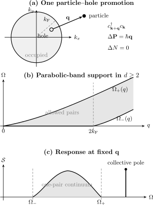
Top: $c_{\mathbf k+\mathbf q}^{\dagger}c_{\mathbf k}$ moves one occupied fermion outside the Fermi sea, leaving a hole with physical momentum $-\hbar\mathbf k$. Middle: in $d\ge2$, allowed parabolic-band transitions fill the region between $\Omega_-(q)$ and $\Omega_+(q)$. Bottom: at fixed $\mathbf q$, a one-body probe sees continuum weight; an interaction can also produce a pole outside it.

Static Structure from Fermi-Sphere Geometry

Equal-time pair count

For $\mathbf q\ne\mathbf0$, the zero-temperature static density structure factor of an ideal gas can be written

$$s_0(q) := \frac1N \sum_{\mathbf k,\sigma} n_{\mathbf k}^{(0)} \left( 1-n_{\mathbf k+\mathbf q}^{(0)} \right).$$

The numerator counts occupied points that leave the Fermi sea after translation by $\mathbf q$. Equivalently, it is the volume of one Fermi sphere minus its overlap with a copy displaced by $q$.

Three-dimensional result

For a spherical three-dimensional sea, the overlap volume of two radius-$k_{\mathrm F}$ spheres separated by $q\le2k_{\mathrm F}$ is

$$V_{\mathrm{overlap}}(q) := \frac{\pi}{12} \left( 4k_{\mathrm F}+q \right) \left( 2k_{\mathrm F}-q \right)^2.$$

Dividing by

$$V_{\mathrm F} := \frac{ 4\pi k_{\mathrm F}^3 }{ 3 }$$

gives

$$s_0(q) := \frac{ 3q }{ 4k_{\mathrm F} } - \frac{ q^3 }{ 16k_{\mathrm F}^3 }, \qquad 0\le q\le2k_{\mathrm F}.$$

For $q\ge2k_{\mathrm F}$ the spheres do not overlap, so

$$s_0(q) := 1.$$

The symbol $s_0$ here is normalized per particle. Some sources instead call the extensive numerator $S_0$ and reserve $S_0/N$ for this result. A quoted formula must identify which convention is meant.

The small-$q$ suppression is Pauli blocking in geometric form:

$$s_0(q) \sim \frac{ 3q }{ 4k_{\mathrm F} }.$$

Only a shell near the Fermi surface can be moved into empty states by a small momentum transfer.

Sum over the continuum

With the energy-resolved convention used above,

$$\int_0^\infty d\Omega\, \mathcal S_\rho^{(0)} \left( \mathbf q,\Omega \right)$$

recovers the equal-time pair count per volume. This is a zeroth-moment check, not a substitute for the full frequency dependence. Structure Factors develops the normalization dictionary and exact moment relations.

Response-Function Bridge

Retarded convention

Define the density response per volume by

$$\chi_{\rho\rho}^R \left( \mathbf q,t \right) := - \frac i{ \hbar\mathcal V } \Theta(t) \left\langle \left[ \rho_{\mathbf q}(t), \rho_{-\mathbf q}(0) \right] \right\rangle.$$

Use an energy transfer $\Omega$ rather than angular frequency:

$$\chi_{\rho\rho}^R \left( \mathbf q,\Omega \right) := \int_{-\infty}^{\infty} dt\, e^{i\Omega t/\hbar} \chi_{\rho\rho}^R \left( \mathbf q,t \right).$$

If a source instead uses $\omega$, substitute $\Omega=\hbar\omega$ and track the corresponding delta-function Jacobian.

Independent-particle polarization

For a spin-degenerate single band,

$$\begin{aligned} \chi_0^R \left( \mathbf q,\Omega \right) :={}& \frac1{\mathcal V} \sum_{\mathbf k,\sigma} \\ &\times \frac{ n_{\mathrm F}(\xi_{\mathbf k}) - n_{\mathrm F}(\xi_{\mathbf k+\mathbf q}) }{ \Omega + \epsilon_{\mathbf k} - \epsilon_{\mathbf k+\mathbf q} + i0^+ }. \end{aligned}$$

This is the independent-particle or Lindhard polarization in the stated sign convention. The numerator enforces occupation availability, while the denominator compares the external energy with the pair energy.

The formula is exact for the independent reference system. It is not by itself an interacting approximation.

Imaginary part counts on-shell pairs

Using

$$\frac1{x+i0^+} := \mathcal P\frac1x - i\pi\delta(x),$$

one finds

$$\begin{aligned} &- \frac1\pi \operatorname{Im} \chi_0^R \left( \mathbf q,\Omega \right) \\ &\quad= \frac1{\mathcal V} \sum_{\mathbf k,\sigma} \\ &\qquad\times \left[ n_{\mathrm F}(\xi_{\mathbf k}) - n_{\mathrm F}(\xi_{\mathbf k+\mathbf q}) \right] \\ &\qquad\times \delta \left( \Omega - \epsilon_{\mathbf k+\mathbf q} + \epsilon_{\mathbf k} \right). \end{aligned}$$

At $T=0$ and $\Omega>0$, every on-shell term has an occupied initial state and an empty final state. Therefore

$$- \frac1\pi \operatorname{Im} \chi_0^R \left( \mathbf q,\Omega \right) := \mathcal S_\rho^{(0)} \left( \mathbf q,\Omega \right) \ge 0.$$

The imaginary part is nonzero precisely where the density operator has on-shell particle–hole transitions.

Fluctuation–dissipation relation

At finite temperature, the unsymmetrized absorption spectrum obeys

$$\mathcal S_\rho \left( \mathbf q,\Omega \right) := - \frac1\pi \frac{ \operatorname{Im} \chi_{\rho\rho}^R \left( \mathbf q,\Omega \right) }{ 1-e^{-\beta\Omega} }.$$

This equation assumes the response and energy-Fourier conventions defined above. Alternative normalizations may move factors of $\pi$, $\hbar$, $N$, or $\mathcal V$.

Detailed balance gives

$$\mathcal S_\rho \left( -\mathbf q,-\Omega \right) := e^{-\beta\Omega} \mathcal S_\rho \left( \mathbf q,\Omega \right).$$

Fluctuation–Dissipation Theorem owns the general proof and convention ledger.

Real and imaginary parts answer different questions

The imaginary part measures absorptive on-shell transitions. The real part is a principal-value sum over virtual transitions:

$$\operatorname{Re} \chi_0^R \left( \mathbf q,\Omega \right) := \frac1{\mathcal V} \mathcal P \sum_{\mathbf k,\sigma} \frac{ n_{\mathbf k} - n_{\mathbf k+\mathbf q} }{ \Omega - \Delta\epsilon_{\mathbf k,\mathbf q} }.$$

Both are required. Static screening can be strong even where no finite-energy absorption occurs, and collective-mode conditions depend on the reactive real part as well as damping from the imaginary part.

Static and uniform limits

At exactly $\mathbf q=\mathbf0$ and $\Omega\ne0$,

$$\chi_{\rho\rho}^R \left( \mathbf0,\Omega \right) := 0$$

for conserved total number.

The thermodynamic static limit is different:

$$\lim_{\mathbf q\to\mathbf0} \chi_{\rho\rho}^R \left( \mathbf q,0 \right) := - \frac{ \partial n }{ \partial\mu }$$

for the common convention in which a positive scalar potential raises the one-particle energy. Reversing the source sign reverses the susceptibility sign. The order of limits must accompany any quoted compressibility relation.

Continuum Edges and Singular Response

Edge weight is dimension dependent

The inequalities $\Omega_-(q)\le\Omega\le\Omega_+(q)$ specify support, not a universal line shape. Near an edge, the response depends on:

• spatial dimension;
• Fermi-surface curvature;
• band velocity at the connected points;
• the probe vertex;
• internal degeneracy;
• temperature and lifetime;
• interactions and vertex corrections.

The same kinematic boundary can produce a step, cusp, square-root feature, divergence, or smooth onset in different systems.

Twice the Fermi Wave Number

For a spherical sea, $q=2k_{\mathrm F}$ connects antipodal points on the Fermi surface. Phase space changes nonanalytically there. The static polarization consequently has a dimension-dependent nonanalyticity, often called a Kohn anomaly.

In real space, nonanalytic structure near $2k_{\mathrm F}$ generates oscillatory long-distance response such as Friedel oscillations. Random Phase Approximation owns explicit Lindhard functions and their screening consequences.

Nesting on a lattice

A lattice Fermi surface may contain extended patches connected by one wave vector $\mathbf Q$. If

$$\epsilon_{\mathbf k+\mathbf Q} \approx \epsilon_{\mathbf k}$$

over a large set of occupied $\mathbf k$, many low-energy pairs share nearly the same momentum. This nesting can enhance density-wave or spin-density-wave response.

Nesting is geometric phase-space enhancement, not by itself proof of an ordered phase. Interaction strength, channel-dependent vertices, competing fluctuations, and dimensionality still matter.

Collective Mode Versus Particle–Hole Continuum

Different spectral structures

A particle–hole continuum is a family of pair transitions. A collective mode is a coherent oscillation involving many microscopic degrees of freedom. In response, an idealized continuum contributes a branch cut or dense set of poles, while a sharp collective mode contributes an isolated pole.

An interacting scalar response often has the schematic form

$$\chi^R := \frac{ \chi_0^R }{ 1-V_{\mathbf q}\chi_0^R },$$

where the precise sign and matrix structure depend on the source and interaction conventions.

A zero of

$$1-V_{\mathbf q}\chi_0^R$$

can create a collective pole even though no corresponding single pair existed in the independent spectrum.

Outside the continuum

If a collective mode lies outside the one-pair continuum, decay into one particle–hole pair is kinematically forbidden. In the idealized approximation it can be sharp:

$$\operatorname{Im} \chi_0^R \left( \mathbf q,\Omega_{\mathrm{mode}} \right) := 0.$$

Examples include a long-wavelength three-dimensional plasmon and zero sound with phase velocity above the relevant quasiparticle velocity.

Inside the continuum

When the mode enters a region where

$$\operatorname{Im} \chi_0^R \ne 0,$$

it can decay into on-shell pairs if the channel and symmetry allow. The pole then moves away from the real axis and acquires Landau damping.

Being outside the one-pair continuum does not guarantee an exactly stable excitation. Multi-pair, phonon, disorder, boundary, and nonlinear decay channels may remain.

Collective Modes owns the general pole, eigenvector, polarization, hybridization, and damping language. Random Phase Approximation derives the direct density-feedback denominator.

How Interactions Reshape the Picture

Fermi-liquid continuation

In a Fermi liquid, the particle and hole near the Fermi surface are dressed quasiparticles rather than bare fermions. Their pair energy is approximately

$$\Omega_{\mathbf k,\mathbf q}^{*} := E_{\mathbf k+\mathbf q}^{*} - E_{\mathbf k}^{*},$$

and the continuum boundaries are correspondingly renormalized by the quasiparticle dispersion.

The response is not obtained by replacing $m$ with $m^*$ everywhere. Quasiparticle residue, interaction vertices, conservation-law Ward identities, and Landau interaction parameters also enter.

Fermi Liquid Theory Preview develops those parameters, the quasiparticle lifetime law, and the collisionless zero-sound equation.

Self-energy and vertex corrections

Interactions modify both propagators and probe vertices:

$$G_0 \longrightarrow G, \qquad \Gamma_0 \longrightarrow \Gamma.$$

A self-energy can shift and broaden the particle and hole. A vertex correction changes how the probe creates the pair and can bind or collectively mix pair configurations.

Keeping dressed propagators while dropping the vertex can violate charge conservation or exact sum rules. Conserved response requires a mutually consistent approximation.

Bound states and resonances

Attractive interaction in a particle–hole channel can pull spectral weight below a continuum edge. A pole below the interband electron–hole continuum is an exciton. In other channels, repeated particle–hole scattering can produce spin waves, paramagnons, density modes, or resonances.

The words “particle–hole excitation” may describe the basis configurations from which such a mode is built, but the resulting eigenmode is not generally one fixed pair.

Multi-pair states

The noninteracting density operator creates one pair directly, but interacting eigenstates are superpositions containing zero, one, and many pair configurations compatible with the conserved quantum numbers.

A two-pair continuum contains states such as

$$c_{p_1}^{\dagger} c_{h_1} c_{p_2}^{\dagger} c_{h_2} \lvert\mathrm{FS}\rangle.$$

Multi-pair support can extend beyond the one-pair boundaries and give a nominally protected collective mode a finite but small lifetime.

Orthogonality catastrophe

A sudden local potential can shake the entire Fermi sea and create arbitrarily many low-energy particle–hole pairs. In the thermodynamic limit, the overlap between the initial and final many-body ground states can vanish.

This is an extreme warning against reducing every neutral excitation to one long-lived pair. The many soft pairs can replace a simple pole by a threshold power law.

Finite Temperature and Nonequilibrium

Thermal occupation factors

At finite temperature there is no single sharply filled pure sea. The absorption weight contains

$$n_{\mathrm F} \left( \xi_{\mathbf k} \right) \left[ 1- n_{\mathrm F} \left( \xi_{\mathbf k+\mathbf q} \right) \right].$$

The first factor is the probability that the initial mode is occupied; the second is the probability that the final mode is available.

Thermal holes already exist below $\mu$, and thermally occupied particles exist above it. Consequently:

• zero-temperature continuum edges acquire exponentially or algebraically small tails;
• negative-energy-transfer processes become possible;
• detailed balance relates absorption and emission;
• Pauli blocking remains but is no longer a sharp step.

Lifetime broadening

If the particle and hole have finite lifetimes, the delta function

$$\delta \left( \Omega-\Delta\epsilon \right)$$

is replaced by a broadened convolution of spectral functions. This softens kinematic edges even at low temperature.

Instrumental resolution produces additional broadening and must not be mistaken for an intrinsic pair lifetime.

Driven distributions

Out of equilibrium, the occupation $n_{\mathbf k}(t)$ need not be a Fermi–Dirac function. Population inversion can reverse the sign of an absorptive contribution and produce gain. A response calculation must then specify:

• the prepared distribution;
• the observation time;
• whether a stationary Fourier transform is meaningful;
• collision and dephasing scales;
• which conservation laws survive the drive.

The algebraic factor $n_{\mathbf k}-n_{\mathbf k+\mathbf q}$ still records occupation imbalance, but equilibrium fluctuation–dissipation relations no longer apply automatically.

Lattice and Multiband Systems

Band-resolved pairs

For Bloch bands $n$ and $m$, the pair energy is

$$\Omega_{mn} \left( \mathbf k,\mathbf q \right) := \epsilon_{m,\mathbf k+\mathbf q} - \epsilon_{n,\mathbf k}.$$

Its occupation weight is

$$n_{\mathrm F} \left( \epsilon_{n,\mathbf k}-\mu \right) \left[ 1- n_{\mathrm F} \left( \epsilon_{m,\mathbf k+\mathbf q}-\mu \right) \right].$$

At zero temperature this enforces an occupied initial Bloch state and an empty final Bloch state.

Crystal momentum is conserved modulo a reciprocal vector:

$$\mathbf k+\mathbf q \equiv \mathbf k' \pmod{\mathbf G}.$$

The continuum is the union of intraband and interband transitions over the Brillouin zone.

Bloch-state form factors

The density vertex is not generally one. It contains a cell-periodic overlap,

Reduce $\mathbf q$ to the first Brillouin zone and retain a reciprocal vector $\mathbf G$ when local-field components matter. A standard density form factor is

$$F_{mn} \left( \mathbf k,\mathbf q+\mathbf G \right) := \left\langle u_{m,\mathbf k+\mathbf q} \middle| e^{i\mathbf G\cdot\mathbf r} \middle| u_{n,\mathbf k} \right\rangle.$$

For $\mathbf G=\mathbf0$, this reduces to the overlap of the cell-periodic Bloch spinors. The precise sign of $\mathbf q$ follows the Fourier convention for the density operator.

The band-resolved spectrum contains

$$\left| F_{mn} \left( \mathbf k,\mathbf q \right) \right|^2.$$

Two bands may have kinematically allowed energy differences but negligible response because orbital, sublattice, spin, or symmetry overlap suppresses the vertex.

Intraband and interband continua

An intraband continuum in a partially filled regular band is usually gapless as $q\to0$. An interband continuum can have a nonzero threshold:

$$\Omega_{\mathrm{inter}}^{\min} \left( \mathbf q \right) := \min_{\mathbf k,n\in\mathrm{occ},m\in\mathrm{empty}} \left[ \epsilon_{m,\mathbf k+\mathbf q} - \epsilon_{n,\mathbf k} \right].$$

In a band insulator, the independent electron–hole threshold is set by the direct or indirect band geometry. Coulomb attraction can place an exciton below that threshold.

Flat bands, Dirac bands, and van Hove points

The parabolic formulas are not universal. A flat band can create large phase space at a narrow energy; a Dirac dispersion changes both boundaries and spinor overlap; a van Hove point can enhance the joint density of states.

For a general dispersion, the reliable procedure is to solve

$$\Omega := \epsilon_{m,\mathbf k+\mathbf q} - \epsilon_{n,\mathbf k}$$

under the occupation and vertex constraints rather than forcing an effective-mass parabola outside its controlled neighborhood.

How Particle–Hole Excitations Are Observed

Scattering probes

Inelastic neutron, x-ray, electron, and atom scattering transfer momentum and energy to the target. After removing probe-specific kinematic and form-factor terms, the intrinsic target information is encoded in a dynamic structure factor or response function.

The measured intensity is not simply the number of kinematically allowed pairs:

$$I_{\mathrm{meas}} \sim \left| M_{\mathrm{probe}} \right|^2 \mathcal S_O \ast R_{\mathrm{instrument}}.$$

Here $M_{\mathrm{probe}}$ contains the coupling and polarization selection rules, while $R_{\mathrm{instrument}}$ denotes energy and momentum resolution.

Bragg spectroscopy of quantum gases

Two laser beams can create a moving optical potential with controlled $(\mathbf q,\Omega)$. The transferred momentum or energy samples a density or spin dynamic structure factor. In a normal degenerate Fermi gas, Pauli blocking and the particle–hole continuum shape the spectrum.

In a paired Fermi gas, the response can additionally contain a collective mode and a pair-breaking continuum. Those are not the same as the normal-state one particle–one hole continuum.

Electron energy-loss spectroscopy

Electron energy-loss spectroscopy commonly measures a loss function of the form

$$\mathcal L \left( \mathbf q,\Omega \right) := - \operatorname{Im} \frac1{ \varepsilon \left( \mathbf q,\Omega \right) }.$$

This can show both particle–hole absorption and collective plasmons, but it is not identical to $-\operatorname{Im}\chi_0$. Electromagnetic screening, geometry, multiple scattering, and matrix elements must be included in a forward model.

Optical and Raman probes

Optical photons carry little crystal momentum on the Brillouin-zone scale, so a direct intraband density transition is strongly constrained near $q=0$. Interband optical transitions can still occur because they change band or orbital character at nearly fixed crystal momentum.

Raman processes can transfer energy and an effective momentum while selecting charge, spin, orbital, or symmetry channels. The observed continuum is therefore vertex resolved.

Single-particle spectroscopy is different

Photoemission and inverse photoemission probe addition and removal spectra:

$$N \longleftrightarrow N\pm1.$$

A density particle–hole excitation remains in the $N$-particle sector. Its continuum is a two-point neutral response, not the same object as a one-particle spectral function.

Interactions can make the two observables communicate: a single-particle quasiparticle may decay by emitting a particle–hole pair, and that process appears in its self-energy. The measured spectra nevertheless have different operator definitions and sum rules.

Important Distinctions

Hole versus antiparticle

A condensed-matter hole is defined relative to occupied fermionic modes in a material or many-body reference. Its energy, charge, and momentum are changes relative to that background.

A relativistic antiparticle is an excitation of a quantum field with its own positive-energy creation operator and transformation laws. Modern quantum field theory does not require interpreting physical antiparticles as literal vacancies in an infinitely filled observable sea.

The algebraic analogy can be useful; the ontological identification is not.

Hole versus particle–hole symmetry

Every partially filled Fermi sea admits hole excitations. Particle–hole symmetry is a much stronger statement: a transformation exchanges creation and annihilation operators while leaving a Hamiltonian or low-energy theory invariant, possibly up to constants and parameter changes.

A generic parabolic electron gas has holes without exact particle–hole symmetry. A lattice model can have an exact particle–hole transformation only at special fillings, lattices, and parameter values.

Pair excitation versus Bogoliubov mixing

An ordinary pair creator is

$$c_p^{\dagger}c_h.$$

It preserves microscopic number and creates a definite addition together with a definite removal.

A fermionic Bogoliubov operator has the form

$$\gamma := u c + v c^{\dagger}.$$

It is a coherent superposition of removal and addition relative to a paired reference and generally does not have a sharp microscopic number change, though fermion parity remains sharp. Bogoliubov Quasiparticles develops that distinction.

Unbound pair versus exciton

An interband electron and hole define a continuum of unbound transitions. An exciton is an interacting bound state, typically appearing as a discrete pole below the continuum threshold.

Seeing an electron and a hole in a basis decomposition does not by itself establish exciton binding. One must compare the pole energy with the continuum edge and show the appropriate two-body or many-body eigenstate.

Continuum versus finite lifetime

A free gas has a broad particle–hole continuum even though every microscopic orbital has infinite lifetime. The continuum width reflects the spread of allowed transition energies.

A finite lifetime broadens each contribution and can smear the edges. These two kinds of width should not be conflated.

Pair continuum versus collective mode

A broad continuum can carry coherent matrix elements, and a collective mode can be damped. “Continuum” and “collective” are not antonyms. The distinction is between a family of pair-like states and a pole whose eigenvector is a coherent many-configuration oscillation.

Role in Many-Body Calculations

Perturbative intermediate states

In a fermionic ground-state expansion, one-body operators generate one-pair states, while two-body interactions can generate up to two pairs at first action:

$$V \lvert\mathrm{FS}\rangle \sim \sum_{ph} V_{ph} \lvert ph^{-1}\rangle + \sum_I V_I \lvert I\rangle,$$

where $I$ indexes a two-particle–two-hole basis state such as

$$\lvert I\rangle := c_{p_1}^{\dagger} c_{p_2}^{\dagger} c_{h_2} c_{h_1} \lvert\mathrm{FS}\rangle.$$

Small particle–hole denominators near a Fermi surface make thermodynamic-limit perturbation theory qualitatively different from a nondegenerate finite-level problem.

Perturbation Theory in Many-Body Systems owns linked-cluster organization, degeneracy, infrared cautions, and size extensivity.

Bubble diagrams

The independent polarization can be represented diagrammatically by a closed fermion loop with two external vertices. One propagator segment carries particle-like time ordering and the other carries hole-like time ordering.

The diagram is a compact bookkeeping device for the same occupation difference and energy denominator derived above. It does not mean that virtual lines are directly observed particles following classical paths.

Diagrammatic Methods Preview owns propagators, vertices, signs, loop counting, and self-energy language.

Quasiparticle decay

An added fermionic quasiparticle can scatter and create an additional particle–hole pair:

$$\mathrm{qp} \longrightarrow \mathrm{qp}' + p + h.$$

Energy, momentum, and Pauli constraints determine the available phase space. Near a regular Fermi surface at low temperature, that phase space is strongly suppressed, helping Landau quasiparticles remain sharp.

The Fermi-surface scaling law belongs with Fermi Liquid Theory Preview, while Lifetime and Spectral Weight owns the general phase-space, width, and validity audit.

Response instabilities

Repeated particle–hole scattering in a channel leads to an integral or matrix eigenvalue problem. A diverging susceptibility can signal that the reference sea is unstable toward:

• charge-density order;
• spin-density order;
• ferromagnetism;
• orbital or valley order;
• an excitonic condensate.

A large bare phase space is one input, not a complete instability proof. The interaction kernel and competing channels decide whether an eigenvalue actually reaches the instability condition.

Reliable Workflow

1. Name the reference. Specify the Fermi sea, mean-field determinant, interacting normal state, band insulator, or nonequilibrium distribution.
2. State the generator. Distinguish $H$ from $H-\mu N$ and define the energy-transfer variable.
3. Fix labels. Say whether a hole is labeled by the removed orbital or by its physical momentum.
4. Write the operator. Identify $c_p^\dagger c_h$ and the full density, spin, current, or orbital vertex.
5. Apply Pauli blocking. Require occupied initial weight and empty final weight.
6. Compute conserved changes. Check number, charge, momentum, spin, parity, and crystal momentum modulo $\mathbf G$.
7. Map support. Optimize the pair energy over all admissible initial states.
8. Compute weight. Include degeneracy, form factors, occupations, and delta-function normalization.
9. Separate response parts. Distinguish absorptive imaginary response from reactive real response.
10. Check limits. Test $q=0$, $q\to0$, $\Omega=0$, $q=2k_{\mathrm F}$, large $q$, and finite size.
11. Add interactions consistently. Treat propagator and vertex corrections in a conservation-compatible scheme.
12. Search for poles. Determine whether interactions bind, collectivize, or damp pair configurations.
13. Model the probe. Fold in polarization, geometry, occupation, detailed balance, and instrumental resolution.
14. Declare the regime. State dimension, band structure, temperature, lifetime, and the range over which the reference is controlled.

Common Mistakes

Calling the hole an extra microscopic particle

A hole is a missing occupation relative to a filled reference. It behaves as an excitation with definite quantum numbers, but its existence and labels depend on that reference.

Giving the hole the removed particle’s momentum

If $d_{\mathbf k}^{\dagger}=c_{\mathbf k}$, then the total momentum change is $-\hbar\mathbf k$. Relabel the hole explicitly if its index is meant to equal physical momentum.

Forgetting Pauli blocking

The energy difference alone does not define an allowed transition. The initial state must carry occupied weight and the final state must carry empty weight.

Treating a continuum as collision broadening

Independent transitions already span a range of energies. Intrinsic lifetimes and disorder broaden those transitions further but do not create the basic continuum.

Assuming every allowed pair is visible

An operator vertex can vanish because of spin, orbital, sublattice, parity, polarization, or destructive-interference selection rules.

Using the three-dimensional boundary in one dimension

For $0<q<2k_{\mathrm F}$, the one-dimensional lower edge is nonzero at fixed $q$. The zero lower edge in $d\ge2$ relies on transverse Fermi-surface geometry.

Confusing exactly zero momentum with a small momentum

The conserved operator $\rho_{\mathbf0}=N$ cannot absorb finite energy. A small but nonzero $\mathbf q$ accesses a thin shell of pair states.

Calling every particle–hole superposition collective

A probe always creates a superposition over allowed pairs. Collectivity requires an interacting eigenmode or response pole with coherent many-configuration structure, not merely a sum in the operator.

Equating particle–hole symmetry with hole excitations

Holes exist generically near a filled occupation boundary. Exact particle–hole symmetry requires a special transformation property of the Hamiltonian.

Calling a normal pair a Bogoliubov quasiparticle

$c_p^\dagger c_h$ preserves number and creates two excitation constituents. $u c+v c^\dagger$ is one canonical quasiparticle operator relative to a paired or anomalous quadratic reference.

Reading the continuum edge as a dispersion branch

The edge is an extremum over many pair states. It need not be an eigenmode that can be followed as a single wave packet.

Dressing propagators but not vertices

In a conserved channel, inconsistent self-energy and vertex approximations can violate continuity equations, Ward identities, and sum rules.

Inferring an instability from nesting alone

Nesting enhances phase space. An instability additionally requires a sufficiently strong attractive eigenvalue in the relevant response channel and must compete with other channels.

Comparing a calculated response directly with raw intensity

Measured spectra include probe matrix elements, thermal factors, geometry, backgrounds, and finite resolution. A forward model is part of the comparison.

Exercises

Exercise 1: Hole dictionary

Consider one occupied mode $h$ with

$$\xi_h < 0,$$

microscopic momentum $\hbar\mathbf h$, and additive charge $q_f$. Define

$$d_h^\dagger := c_h.$$

Show that the hole has positive grand-canonical energy, momentum change $-\hbar\mathbf h$, and charge change $-q_f$.

Solution

The mode contribution to the grand generator is

$$K_h := \xi_h c_h^\dagger c_h.$$

Since

$$d_h^\dagger d_h := c_h c_h^\dagger := 1-c_h^\dagger c_h,$$

we obtain

$$K_h := \xi_h + \left( -\xi_h \right) d_h^\dagger d_h.$$

The coefficient of the hole number is therefore

$$E_h := -\xi_h > 0.$$

For momentum,

$$\left[ \mathbf P, d_h^\dagger \right] := \left[ \mathbf P, c_h \right] := -\hbar\mathbf h\, d_h^\dagger.$$

Thus the hole changes the system momentum by $-\hbar\mathbf h$.

If

$$Q := \sum_j q_f c_j^\dagger c_j,$$

then

$$\left[ Q, d_h^\dagger \right] := -q_f d_h^\dagger.$$

Removing one microscopic charge $q_f$ creates an excitation with charge change $-q_f$.

Exercise 2: Norm and quantum numbers of one pair

Let $h$ be occupied and $p$ empty in $\lvert\mathrm{FS}\rangle$. For

$$\lvert ph^{-1}\rangle := c_p^\dagger c_h \lvert\mathrm{FS}\rangle,$$

show that the state has unit norm, preserves total number, and has independent-particle energy $\epsilon_p-\epsilon_h$.

Solution

The norm is

$$\begin{aligned} \langle ph^{-1}\vert ph^{-1}\rangle ={}& \langle\mathrm{FS}\rvert c_h^\dagger c_p c_p^\dagger c_h \lvert\mathrm{FS}\rangle \\ ={}& \langle\mathrm{FS}\rvert c_h^\dagger \left( 1-c_p^\dagger c_p \right) c_h \lvert\mathrm{FS}\rangle \\ ={}& n_h^{(0)} \left( 1-n_p^{(0)} \right) \\ ={}& 1. \end{aligned}$$

The number commutator is

$$\begin{aligned} \left[ N, c_p^\dagger c_h \right] &= \left[ N,c_p^\dagger \right] c_h + c_p^\dagger \left[ N,c_h \right] \\ &= c_p^\dagger c_h - c_p^\dagger c_h \\ &= 0. \end{aligned}$$

For

$$H_0 := \sum_j \epsilon_j c_j^\dagger c_j,$$

we have

$$\left[ H_0, c_p^\dagger c_h \right] := \left( \epsilon_p-\epsilon_h \right) c_p^\dagger c_h.$$

Therefore the normalized pair state has energy $\epsilon_p-\epsilon_h$ above the Fermi sea.

Exercise 3: Continuum boundaries in two and higher dimensions

For

$$\epsilon_{\mathbf k} := \frac{ \hbar^2k^2 }{ 2m },$$

derive the upper continuum edge and explain geometrically why the lower edge vanishes for $0<q<2k_{\mathrm F}$ when $d\ge2$.

Solution

Choose $\mathbf q$ as the longitudinal axis. The transfer is

$$\Omega_{\mathbf k,\mathbf q} := \frac{ \hbar^2q^2 }{ 2m } + \frac{ \hbar^2kq }{ m } \cos\theta.$$

The maximum uses the largest occupied $k$ and $\cos\theta=1$:

$$k \to k_{\mathrm F}, \qquad \Omega_+(q) := \frac{ \hbar^2q^2 }{ 2m } + \hbar v_{\mathrm F}q.$$

For $q<2k_{\mathrm F}$, the original Fermi sphere and a copy shifted by $-\mathbf q$ intersect in a $(d-2)$-dimensional set. Choose an initial point infinitesimally inside the original sphere near that intersection. Its translated final point can be infinitesimally outside the sphere. Hence

$$\epsilon_{\mathbf k+\mathbf q} - \epsilon_{\mathbf k} \to 0^+.$$

Therefore

$$\Omega_-(q) := 0, \qquad 0<q\le2k_{\mathrm F}.$$

For $q>2k_{\mathrm F}$, the minimum occurs at $\mathbf k=-k_{\mathrm F}\widehat{\mathbf q}$:

$$\Omega_-(q) := \frac{ \hbar^2q^2 }{ 2m } - \hbar v_{\mathrm F}q.$$

Exercise 4: One-dimensional continuum

Take $q>0$ in a one-dimensional ideal Fermi gas with occupied interval

$$-k_{\mathrm F} \le k \le k_{\mathrm F}.$$

Derive the allowed interval of initial $k$ and the continuum edges for $0<q<2k_{\mathrm F}$.

Solution

The final state $k+q$ must lie above the right Fermi point because $q>0$. Thus

$$k+q > k_{\mathrm F},$$

while the initial point remains occupied. For $0<q<2k_{\mathrm F}$,

$$k_{\mathrm F}-q < k \le k_{\mathrm F}.$$

The transfer

$$\Omega(k,q) := \frac{ \hbar^2 }{ 2m } \left[ \left( k+q \right)^2-k^2 \right]$$

is linear in $k$:

$$\Omega(k,q) := \frac{ \hbar^2q^2 }{ 2m } + \frac{ \hbar^2kq }{ m }.$$

The minimum occurs at $k=k_{\mathrm F}-q$:

$$\Omega_-^{(1\mathrm D)} := \hbar v_{\mathrm F}q - \frac{ \hbar^2q^2 }{ 2m }.$$

The maximum occurs at $k=k_{\mathrm F}$:

$$\Omega_+^{(1\mathrm D)} := \hbar v_{\mathrm F}q + \frac{ \hbar^2q^2 }{ 2m }.$$

At fixed nonzero $q<2k_{\mathrm F}$, the lower edge is positive. Both edges approach $\hbar v_{\mathrm F}q$ in the long-wavelength limit.

Exercise 5: Static structure factor from overlapping spheres

Two spheres of radius $R$ whose centers are separated by $q\le2R$ have overlap volume

$$V_{\mathrm{overlap}} := \frac{\pi}{12} \left( 4R+q \right) \left( 2R-q \right)^2.$$

Use this result to derive the per-particle static structure factor of a three-dimensional ideal Fermi gas.

Solution

The Fermi-sphere volume is

$$V_{\mathrm F} := \frac{ 4\pi R^3 }{ 3 }.$$

The fraction of occupied initial states that remain inside after translation is the overlap fraction:

$$\frac{ V_{\mathrm{overlap}} }{ V_{\mathrm F} } := \frac{ \left( 4R+q \right) \left( 2R-q \right)^2 }{ 16R^3 }.$$

The fraction promoted outside is one minus this overlap. Setting $R=k_{\mathrm F}$ and expanding,

$$\begin{aligned} s_0(q) &:= 1- \frac{ V_{\mathrm{overlap}} }{ V_{\mathrm F} } \\ &= \frac{ 3q }{ 4k_{\mathrm F} } - \frac{ q^3 }{ 16k_{\mathrm F}^3 }, \qquad q\le2k_{\mathrm F}. \end{aligned}$$

For $q\ge2k_{\mathrm F}$, the spheres do not overlap, so

$$s_0(q) := 1.$$

The internal degeneracy cancels between the number of promoted states and the total particle number.

Exercise 6: Sign of the absorptive response

Starting from

$$\chi_0^R \left( \mathbf q,\Omega \right) := \frac1{\mathcal V} \sum_{\mathbf k,\sigma} \frac{ n_{\mathbf k}-n_{\mathbf k+\mathbf q} }{ \Omega-\Delta\epsilon_{\mathbf k,\mathbf q}+i0^+ },$$

show that $\operatorname{Im}\chi_0^R\le0$ for $\Omega>0$ at zero temperature.

Solution

The distribution identity gives

$$\begin{aligned} \operatorname{Im} \chi_0^R \left( \mathbf q,\Omega \right) :={}& - \frac{\pi}{\mathcal V} \sum_{\mathbf k,\sigma} \left( n_{\mathbf k} - n_{\mathbf k+\mathbf q} \right) \\ &\times \delta \left( \Omega - \Delta\epsilon_{\mathbf k,\mathbf q} \right). \end{aligned}$$

For $\Omega>0$, the delta function requires a positive energy transfer. At zero temperature, an allowed absorptive transition has

$$n_{\mathbf k} := 1, \qquad n_{\mathbf k+\mathbf q} := 0.$$

Every nonzero summand inside the brackets is therefore positive. The explicit minus sign implies

$$\operatorname{Im} \chi_0^R \le 0.$$

Consequently,

$$- \frac1\pi \operatorname{Im} \chi_0^R$$

is a nonnegative absorption spectrum in this convention.

Exercise 7: Exactly uniform versus long wavelength

Explain why

$$\chi_{\rho\rho}^R \left( \mathbf0,\Omega \right) := 0$$

for $\Omega\ne0$ in a number-conserving system, while the static limit $\mathbf q\to0$ can remain finite.

Solution

At exactly zero momentum,

$$\rho_{\mathbf0} := N.$$

If

$$\left[ H,N \right] := 0,$$

then $N(t)=N$ and

$$\left[ N(t),N(0) \right] := 0.$$

The retarded correlator therefore vanishes at every nonzero frequency:

$$\chi_{\rho\rho}^R \left( \mathbf0,\Omega \right) := 0.$$

For small but nonzero $\mathbf q$, $\rho_{\mathbf q}$ is not the conserved total number. It transfers momentum and creates particle–hole pairs in a thin shell near the Fermi surface.

The static protocol also allows the density to re-equilibrate under a spatially slowly varying source. With the source convention used on this page,

$$\lim_{\mathbf q\to0} \chi_{\rho\rho}^R \left( \mathbf q,0 \right) := - \frac{ \partial n }{ \partial\mu },$$

which is finite for a compressible Fermi gas. The two expressions describe different orders of limits and different physical protocols.

Exercise 8: Pole placement and damping

At fixed $q$, suppose the one-pair continuum occupies

$$\Omega_-(q) \le \Omega \le \Omega_+(q).$$

Classify the leading one-pair damping of three collective solutions:

1. $\Omega_a>\Omega_+$;
2. $\Omega_-<\Omega_b<\Omega_+$;
3. $0<\Omega_c<\Omega_-$ for a momentum where $\Omega_->0$.

State one reason that a mode outside the one-pair continuum may still have finite lifetime.

Solution

For modes $a$ and $c$,

$$\operatorname{Im} \chi_0^R \left( q,\Omega_{a,c} \right) := 0$$

in the ideal zero-temperature one-pair approximation. Decay into one particle–hole pair is kinematically forbidden.

For mode $b$,

$$\operatorname{Im} \chi_0^R \left( q,\Omega_b \right) \ne 0$$

provided the operator channel has nonzero matrix element. The collective pole can decay into on-shell particle–hole states and acquires Landau damping.

Modes $a$ and $c$ are protected only against this one channel. They can still decay through:

• two or more particle–hole pairs;
• phonons or other collective modes;
• disorder or boundaries;
• nonlinear coupling;
• thermal scattering.

Thus “outside the continuum” is a channel-specific kinematic statement, not a proof of exact stability.

Key Takeaways

• A particle–hole excitation moves one fermion from occupied to empty one-particle weight and preserves total microscopic number.
• The hole is a missing occupation; when labeled by the removed momentum $\mathbf k$, its physical momentum change is $-\hbar\mathbf k$.
• Pauli blocking is the factor $n_h(1-n_p)$ and is already enforced by fermionic operator algebra.
• At fixed transferred momentum, many allowed initial states produce a continuum of pair energies in the thermodynamic limit.
• For an isotropic parabolic band in $d\ge2$, the continuum extends from $\max(0,\hbar^2q^2/2m-\hbar v_{\mathrm F}q)$ to $\hbar^2q^2/2m+\hbar v_{\mathrm F}q$.
• In one dimension the lower edge is generally nonzero at fixed $0<q<2k_{\mathrm F}$ because there is no transverse Fermi-surface geometry.
• The imaginary part of the independent retarded response counts on-shell pair transitions; the real part records virtual transitions and controls screening and collective-mode conditions.
• A continuum exists without collisions. Lifetime broadening, thermal smearing, disorder, and instrumental resolution are additional effects.
• Interactions can dress, bind, collectivize, or multiply particle–hole configurations.
• Hole excitations, exact particle–hole symmetry, Bogoliubov mixing, excitons, antiparticles, and single-particle spectra are related ideas but not interchangeable.

References and Further Reading

1. J. Lindhard, “On the Properties of a Gas of Charged Particles,” Kongelige Danske Videnskabernes Selskab, Matematisk-fysiske Meddelelser 28, no. 8, 1–57 (1954), OSTI record. Original independent-electron dielectric response and polarization treatment.
2. D. Bohm and D. Pines, “A Collective Description of Electron Interactions. II. Collective vs Individual Particle Aspects of the Interactions,” Physical Review 85, 338–353 (1952), doi:10.1103/PhysRev.85.338. Foundational separation of collective and individual electronic response.
3. D. Bohm and D. Pines, “A Collective Description of Electron Interactions. III. Coulomb Interactions in a Degenerate Electron Gas,” Physical Review 92, 609–625 (1953), doi:10.1103/PhysRev.92.609. Collective modes, screened interactions, and the degenerate electron gas.
4. L. Van Hove, “Correlations in Space and Time and Born Approximation Scattering in Systems of Interacting Particles,” Physical Review 95, 249–262 (1954), doi:10.1103/PhysRev.95.249. Correlation functions and scattering spectra.
5. R. Kubo, “Statistical-Mechanical Theory of Irreversible Processes. I,” Journal of the Physical Society of Japan 12, 570–586 (1957), doi:10.1143/JPSJ.12.570. Retarded response and fluctuation–dissipation foundations.
6. F. Stern, “Polarizability of a Two-Dimensional Electron Gas,” Physical Review Letters 18, 546–548 (1967), doi:10.1103/PhysRevLett.18.546. Canonical two-dimensional polarization and plasmon analysis.
7. P. W. Anderson, “Infrared Catastrophe in Fermi Gases with Local Scattering Potentials,” Physical Review Letters 18, 1049–1051 (1967), doi:10.1103/PhysRevLett.18.1049. Many-soft-pair response and vanishing ground-state overlap.
8. P. Nozières and C. T. De Dominicis, “Singularities in the X-Ray Absorption and Emission of Metals. III. One-Body Theory Exact Solution,” Physical Review 178, 1097–1107 (1969), doi:10.1103/PhysRev.178.1097. Threshold spectra generated by a Fermi sea of particle–hole excitations.
9. A. L. Fetter and J. D. Walecka, Quantum Theory of Many-Particle Systems (McGraw–Hill, 1971; Dover reprint, 2003). Standard operator, response, electron-gas, and collective-mode treatment.
10. D. Pines and P. Nozières, The Theory of Quantum Liquids, Volume I: Normal Fermi Liquids (W. A. Benjamin, 1966; CRC reprint, 2018). Particle–hole response and Fermi-liquid foundations.
11. G. D. Mahan, Many-Particle Physics, 2nd ed. (Plenum, 1990), doi:10.1007/978-1-4613-1469-1. Green functions, Lindhard response, screening, and spectroscopy.
12. G. F. Giuliani and G. Vignale, Quantum Theory of the Electron Liquid (Cambridge University Press, 2005), doi:10.1017/CBO9780511619915. Modern electron-liquid response across dimensions.
13. H. Bruus and K. Flensberg, Many-Body Quantum Theory in Condensed Matter Physics (Oxford University Press, 2004), doi:10.1093/acprof:oso/9780198566335.001.0001. Pedagogical second-quantized and response treatment.
14. G. Veeravalli, E. Kuhnle, P. Dyke, and C. J. Vale, “Bragg Spectroscopy of a Strongly Interacting Fermi Gas,” Physical Review Letters 101, 250403 (2008), doi:10.1103/PhysRevLett.101.250403. Experimental dynamic and static structure-factor spectroscopy in a Fermi gas.
15. S. Giorgini, L. P. Pitaevskii, and S. Stringari, “Theory of Ultracold Atomic Fermi Gases,” Reviews of Modern Physics 80, 1215–1274 (2008), doi:10.1103/RevModPhys.80.1215. Authoritative review of normal and paired atomic Fermi gases.