Magnons

A magnon is one quantum of a spin-wave normal mode about an ordered magnetic reference state. The microscopic variables are fixed-length quantum spins, but the low-amplitude transverse deviations of an ordered texture behave as coupled bosonic coordinates. Diagonalizing their quadratic dynamics gives spin-wave modes; quantizing those modes gives magnons.

The conceptual chain is

$$\begin{gathered} \text{ordered magnetic reference}, \\ \downarrow \\ \text{small transverse spin deviations}, \\ \downarrow \\ \text{spin-wave normal modes}, \\ \downarrow \\ \text{magnon quanta}. \end{gathered}$$

This separates three related objects:

• a spin-wave mode is an allowed normal pattern of transverse motion;
• a magnon is one quantum occupying a spin-wave mode;
• a classical precessing spin wave is usually represented by a coherent state with an indefinite, often large, magnon occupation.

A localized spin flip is not generally an energy eigenstate. Exchange transports and phase-locks spin deviations, so a one-magnon eigenstate is usually spread over many sites. Conversely, a single magnon number state has no classical transverse magnetization expectation value. It is detected through its energy, momentum, angular-momentum transfer, fluctuations, and transition matrix elements.

Magnons are bosonic quasiparticles even though a spin has only $2s+1$ local states. The bosonic representation is exact only after restricting each auxiliary oscillator to a finite physical subspace. Linear spin-wave theory then replaces that constrained problem by a dilute, approximately unconstrained boson theory. Its reliability depends on the ordered reference, the spin-deviation density, dimensionality, interactions, and the observable being computed.

Scope and Canonical Ownership

This page owns the general spin-wave quantization framework:

• local frames around collinear and slowly varying magnetic order;
• the exact Holstein–Primakoff representation and its physical subspace;
• the low-density expansion leading to linear spin-wave theory;
• generic ferromagnetic and bipartite-antiferromagnetic quadratic Hamiltonians;
• number-conserving versus anomalous bosonic terms;
• quadratic versus linear long-wavelength dispersions;
• magnon momentum, spin polarization, coherent waves, and probe matrix elements;
• zero-point and thermal spin reduction;
• the origin of magnon interactions, decay, and quasiparticle breakdown;
• practical validity checks and common convention traps.

Neighboring pages keep more specialized ownership:

• Spin as Intrinsic Angular Momentum owns the local spin algebra and finite spin-$s$ representation.
• Spin Rotations owns active and passive rotation conventions.
• Heisenberg Model owns the isotropic exchange model, its sign convention, exact one-magnon chain result, and model-specific benchmarks.
• Exchange Interactions in Quantum Matter owns the microscopic material pathways and experimental extraction of the couplings that set magnon dispersions.
• Spin Waves and Magnons in Materials owns the magnetic-structure ledger, material Hamiltonian, probe-weighted forward model, resolution treatment, and parameter-validation workflow.
• Bosonic Operators in Many-Body Models owns abstract bosonic Fock-space algebra.
• Collective Modes owns the cross-system normal-mode and response-eigenchannel framework.
• Goldstone Modes in Many-Body Systems owns broken-generator counting and the type-A versus type-B classification.
• Bogoliubov Theory owns the general paraunitary diagonalization of stable quadratic bosonic Hamiltonians.
• Structure Factors owns exact scattering normalizations, spectral representations, detailed balance, and sum rules.
• Spectral Functions owns pole, residue, linewidth, continuum, and self-energy conventions.

Material-specific exchange networks, magnetic domains, first-principles parameters, magnonic devices, and phase claims begin at Magnetism and Spin Systems. The gateway chooses the material branch; the aim here remains the reusable excitation theory that connects an ordered spin Hamiltonian to its harmonic bosons.

Spin and Fourier Conventions

Dimensionless spin operators

At site $i$, use dimensionless spin operators $\mathbf s_i$:

$$\begin{aligned} \left[ s_i^\alpha, s_j^\beta \right] &:= i\delta_{ij} \epsilon_{\alpha\beta\gamma} s_i^\gamma, \\ \mathbf s_i^2 &:= s(s+1). \end{aligned}$$

Physical angular momentum is

$$\mathbf S_i := \hbar\mathbf s_i.$$

The ladder operators are

$$s_i^\pm := s_i^x \pm i s_i^y,$$

and obey

$$\left[ s_i^z,s_i^\pm \right] := \pm s_i^\pm.$$

An energy denoted $\varepsilon_{\mathbf q\nu}$ corresponds to angular frequency

$$\omega_{\mathbf q\nu} := \frac{ \varepsilon_{\mathbf q\nu} }{ \hbar }.$$

Keeping energy and angular frequency distinct prevents missing factors of $\hbar$ in response functions and equations of motion.

Lattice Fourier transform

For a Bravais lattice with $N$ sites and positions $\mathbf R_i$, use

$$\begin{aligned} a_{\mathbf q} &:= \frac{1}{\sqrt N} \sum_i e^{-i\mathbf q\cdot\mathbf R_i} a_i, \\ a_i &:= \frac{1}{\sqrt N} \sum_{\mathbf q} e^{i\mathbf q\cdot\mathbf R_i} a_{\mathbf q}. \end{aligned}$$

Then

$$\left[ a_{\mathbf q}, a_{\mathbf q'}^\dagger \right] := \delta_{\mathbf q,\mathbf q'}.$$

For a bipartite antiferromagnet, separate transforms on the $A$ and $B$ sublattices are more transparent. Momentum may then be restricted to a magnetic Brillouin zone. A full-zone convention can display the same degrees of freedom as symmetry-related soft points instead. Branch counts must therefore be stated together with the zone convention.

Ordered Reference States

Why a reference is needed

Spin-wave theory is an expansion around an ordered texture

$$\left\{ \mathbf n_i^{\,0} \right\}, \qquad \left| \mathbf n_i^{\,0} \right| := 1.$$

The classical reference moment is

$$\left\langle \mathbf s_i \right\rangle_{\mathrm{cl}} := s\mathbf n_i^{\,0}.$$

This reference may be:

• a uniform ferromagnet;
• a two-sublattice collinear antiferromagnet;
• a ferrimagnet with unequal sublattices;
• a spiral or other noncollinear order;
• a field-polarized state;
• a texture that varies slowly compared with the lattice spacing.

The existence of a classical stationary point is not enough. The ordered phase must survive quantum and thermal fluctuations on the scales of interest, and the quadratic fluctuation spectrum must be dynamically stable.

Local axes

Choose an orthonormal triad at every site:

$$\left( \mathbf e_i^1, \mathbf e_i^2, \mathbf e_i^3 \right), \qquad \mathbf e_i^3 := \mathbf n_i^{\,0}.$$

Resolve the physical spin into local components:

$$\mathbf s_i := \sum_{a=1}^{3} \mathbf e_i^a \widetilde s_i^a.$$

The local longitudinal component $\widetilde s_i^3$ points along the ordered moment even when physical moments on different sublattices point in opposite directions. This local rotation is essential in antiferromagnets: applying one global Holstein–Primakoff map to up and down spins without rotating axes produces incorrect signs and an unstable expansion.

For a general spin Hamiltonian,

$$H := H\left( \left\{ \mathbf s_i \right\} \right),$$

the expansion has the schematic large-$s$ hierarchy

$$\begin{aligned} H &:= E_{\mathrm{cl}} + H^{[1]} + H^{[2]} \\ &\quad + H^{[3]} + H^{[4]} + \cdots. \end{aligned}$$

Here $H^{[n]}$ contains $n$ bosonic fluctuation operators after expanding square roots. A correctly chosen stationary reference makes

$$H^{[1]} := 0.$$

Nonzero linear terms are not harmless: they mean the proposed reference is not stationary under the Hamiltonian and constraints being used.

The Exact Holstein–Primakoff Map

One spin as a constrained oscillator

For a spin locally aligned with $+z$, introduce a boson $a_i$ with

$$n_i := a_i^\dagger a_i.$$

The exact Holstein–Primakoff representation is

$$\begin{aligned} \widetilde s_i^z &:= s-n_i, \\ \widetilde s_i^+ &:= \sqrt{ 2s-n_i } \,a_i, \\ \widetilde s_i^- &:= a_i^\dagger \sqrt{ 2s-n_i }. \end{aligned}$$

The physical subspace is

$$\mathcal H_{i,\mathrm{phys}} := \operatorname{span} \left\{ \lvert n_i\rangle: 0\leq n_i\leq 2s \right\}.$$

It has dimension $2s+1$, exactly matching the spin Hilbert space. The identification is

$$\lvert s,m\rangle_i \longleftrightarrow \lvert n_i=s-m\rangle.$$

The square roots produce the correct finite-spin matrix elements:

$$\begin{aligned} \widetilde s_i^+ \lvert n\rangle &:= \sqrt{ n(2s-n+1) } \lvert n-1\rangle, \\ \widetilde s_i^- \lvert n\rangle &:= \sqrt{ (n+1)(2s-n) } \lvert n+1\rangle. \end{aligned}$$

At $n=2s$, the lowering matrix element vanishes. The oscillator state $\lvert 2s+1\rangle$ is unphysical and must not be reached by the exact spin operators.

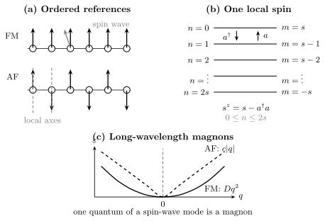
Spin-wave quantization starts from an ordered reference, maps local spin deviations to constrained bosons, and diagonalizes their coupled quadratic dynamics. An isotropic ferromagnet has a quadratic long-wavelength magnon, whereas a collinear antiferromagnet has linear transverse modes.

Why the ordering matters

Because $n_i$ and $a_i$ do not commute, the square-root placement is part of the definition. For example,

$$\sqrt{2s-n_i}\,a_i \neq a_i\sqrt{2s-n_i}.$$

Changing the order shifts the number inside the square root and gives the wrong ladder matrix elements. The exact representation should be checked by its action on $\lvert n\rangle$, not by treating $n_i$ as an ordinary number too early.

Low-density expansion

For

$$\frac{ \langle n_i\rangle }{ 2s } \ll 1,$$

expand

$$\begin{aligned} \sqrt{ 2s-n_i } &:= \sqrt{2s} \Bigg[ 1 - \frac{n_i}{4s} \\ &\qquad - \frac{n_i^2}{32s^2} - \cdots \Bigg]. \end{aligned}$$

At leading order,

$$\begin{aligned} \widetilde s_i^z &:= s-a_i^\dagger a_i, \\ \widetilde s_i^+ &\simeq \sqrt{2s}\,a_i, \\ \widetilde s_i^- &\simeq \sqrt{2s}\,a_i^\dagger. \end{aligned}$$

Equivalently,

$$\begin{aligned} \widetilde s_i^x &\simeq \sqrt{\frac{s}{2}} \left( a_i+a_i^\dagger \right), \\ \widetilde s_i^y &\simeq -i \sqrt{\frac{s}{2}} \left( a_i-a_i^\dagger \right). \end{aligned}$$

The longitudinal deviation is quadratic in bosons while transverse deviations are linear. This is why transverse spin correlations couple directly to one-magnon states, whereas longitudinal correlations begin with two-magnon or density-like processes in a collinear magnet.

What is exact and what is approximate

Three logically separate steps are often called “the Holstein–Primakoff approximation”:

1. The map itself is exact on the constrained physical subspace.
2. Expanding the square root is a controlled low-density or large-$s$ approximation.
3. Keeping only $H^{[2]}$ is linear spin-wave theory.

Diagonalizing $H^{[2]}$ exactly does not restore $H^{[3]}$, $H^{[4]}$, or the local occupancy constraint. A stable quadratic spectrum is necessary but not sufficient for quantitative accuracy.

Linear Spin-Wave Theory

Harmonic truncation

After local rotations and the Holstein–Primakoff expansion, linear spin-wave theory retains

$$H_{\mathrm{LSW}} := E_{\mathrm{cl}} + H^{[2]}.$$

The generic translation-invariant quadratic Hamiltonian is

$$\begin{aligned} H^{[2]} := E_2 &+ \sum_{\mathbf q} a_{\mathbf q}^\dagger A(\mathbf q) a_{\mathbf q} \\ &+ \frac12 \sum_{\mathbf q} \left[ a_{\mathbf q}^\dagger B(\mathbf q) a_{-\mathbf q}^\dagger + \mathrm{h.c.} \right], \end{aligned}$$

with matrix-valued $A$ and $B$ when there are several spins in the magnetic unit cell. Normal terms conserve auxiliary boson number. Anomalous terms create or annihilate boson pairs and require a bosonic Bogoliubov transformation.

The calculation is trustworthy only after checking:

• all classical torque equations, so $H^{[1]}=0$;
• Hermiticity and the bosonic symmetry of the anomalous block;
• positive-norm, real-frequency modes of the bosonic dynamical matrix;
• correct treatment of exact zero modes;
• convergence of zero-point and thermal spin-deviation densities;
• small occupation relative to $2s$;
• robustness under system size and momentum resolution.

Ferromagnetic Magnons

Exchange convention

To isolate the ferromagnetic structure without colliding with other sign conventions, define

$$H_{\mathrm F} := - \frac12 \sum_{i,j} J_{ij} \mathbf s_i\cdot\mathbf s_j - h \sum_i s_i^z,$$

where

$$J_{ij} := J_{ji}, \qquad J_{ii} := 0,$$

and the relevant couplings favor parallel alignment. The factor $1/2$ compensates for summing each unordered pair twice. The Zeeman energy $h$ is positive when the field favors $+z$.

For a translation-invariant Bravais lattice, write

$$J_{ij} := J(\mathbf R_i-\mathbf R_j)$$

and define

$$J(\mathbf q) := \sum_{\mathbf R} J(\mathbf R) e^{i\mathbf q\cdot\mathbf R}.$$

For inversion-symmetric exchange, $J(\mathbf q)$ is real.

Quadratic Hamiltonian

With all moments aligned along $+z$,

$$\mathbf s_i\cdot\mathbf s_j := s_i^zs_j^z + \frac12 \left( s_i^+s_j^- + s_i^-s_j^+ \right).$$

To quadratic order,

$$\begin{aligned} \mathbf s_i\cdot\mathbf s_j \simeq s^2 &- s \left( n_i+n_j \right) \\ &+ s \left( a_i^\dagger a_j + a_j^\dagger a_i \right). \end{aligned}$$

Fourier transformation gives

$$H_{\mathrm F}^{[2]} := E_{\mathrm F} + \sum_{\mathbf q} \varepsilon_{\mathrm F}(\mathbf q) a_{\mathbf q}^\dagger a_{\mathbf q},$$

with

$$\varepsilon_{\mathrm F}(\mathbf q) := h + s \left[ J(\mathbf 0)-J(\mathbf q) \right].$$

There are no anomalous terms. Axial spin conservation makes a spin deviation a number-conserving excitation in this collinear reference.

Nearest-neighbor chain

For a chain with spacing $a$ and ferromagnetic coupling $J_{\mathrm F}>0$ to the two nearest neighbors,

$$J(q) := 2J_{\mathrm F}\cos(qa).$$

Therefore

$$\varepsilon_{\mathrm F}(q) := h + 2sJ_{\mathrm F} \left[ 1-\cos(qa) \right].$$

At $h=0$ and small $q$,

$$\varepsilon_{\mathrm F}(q) \simeq sJ_{\mathrm F}a^2q^2.$$

This agrees with the exact one-magnon result in the isotropic ferromagnetic chain. The Heisenberg Model gives that exact lattice derivation in its own exchange convention.

Long-wavelength stiffness

If $J(\mathbf R)=J(-\mathbf R)$ and the second moment exists,

$$J(\mathbf 0)-J(\mathbf q) \simeq \frac12 \sum_{\mathbf R} J(\mathbf R) \left( \mathbf q\cdot\mathbf R \right)^2.$$

Hence

$$\varepsilon_{\mathrm F}(\mathbf q) \simeq h + \rho_{\alpha\beta} q_\alpha q_\beta,$$

where

$$\rho_{\alpha\beta} := \frac{s}{2} \sum_{\mathbf R} J(\mathbf R) R_\alpha R_\beta.$$

For an isotropic medium,

$$\rho_{\alpha\beta} := \rho\,\delta_{\alpha\beta}.$$

At zero field, the quadratic dispersion is the characteristic type-B Goldstone behavior of an isotropic ferromagnet. The two transverse components are canonically conjugate and form one propagating magnon mode, rather than two independent linearly dispersing polarizations.

One-magnon states

The fully polarized state $\lvert F\rangle$ is the Holstein–Primakoff vacuum:

$$a_i\lvert F\rangle := 0.$$

A momentum eigenstate is

$$\lvert \mathbf q\rangle := a_{\mathbf q}^\dagger \lvert F\rangle \simeq \frac{1}{\sqrt{2sN}} \sum_j e^{i\mathbf q\cdot\mathbf R_j} s_j^- \lvert F\rangle.$$

It is a coherent spatial superposition of one local spin deviation. In an isotropic Heisenberg ferromagnet, the one-deviation sector is closed, so this one-magnon dispersion is exact even though interactions matter in sectors with two or more magnons.

At $h=0$,

$$a_{\mathbf 0}^\dagger \lvert F\rangle \propto s_{\mathrm{tot}}^- \lvert F\rangle.$$

This state lies in the same maximal-spin ground multiplet. On a finite system it is a global rotation, not the first nonuniform propagating wave. The lowest dispersing mode has nonzero momentum and, for a box of size $L$, typically scales as $L^{-2}$.

Bipartite Antiferromagnetic Magnons

Néel reference and local rotation

Consider the nearest-neighbor model

$$H_{\mathrm{AF}} := J \sum_{ \langle i\in A,j\in B\rangle } \mathbf s_i\cdot\mathbf s_j, \qquad J>0.$$

The classical Néel reference points along $+z$ on $A$ and $-z$ on $B$. Rotate each $B$-sublattice spin by $\pi$ about its local $y$ axis:

$$\begin{aligned} s_j^x &:= -\widetilde s_j^x, \\ s_j^y &:= \widetilde s_j^y, \\ s_j^z &:= -\widetilde s_j^z. \end{aligned}$$

Both local reference moments now point along local $+\widetilde z$. For one $A$–$B$ bond,

$$\mathbf s_i\cdot\mathbf s_j := - s_i^z\widetilde s_j^z - \frac12 \left( s_i^+\widetilde s_j^+ + s_i^-\widetilde s_j^- \right).$$

Introduce $a_i$ on $A$ and $b_j$ on $B$. To quadratic order,

$$\begin{aligned} \mathbf s_i\cdot\mathbf s_j \simeq -s^2 &+ s \left( a_i^\dagger a_i + b_j^\dagger b_j \right) \\ &- s \left( a_i b_j + a_i^\dagger b_j^\dagger \right). \end{aligned}$$

The pair terms are the central difference from the ferromagnet. A local deviation on each sublattice changes the physical uniform spin in opposite directions, so creating one $A$ boson and one $B$ boson can preserve the conserved total $s^z$.

Magnetic-zone Hamiltonian

Let $z$ be the coordination number and

$$\gamma_{\mathbf q} := \frac1z \sum_{\boldsymbol\delta} e^{i\mathbf q\cdot\boldsymbol\delta},$$

where $\boldsymbol\delta$ runs from an $A$ site to its $z$ neighboring $B$ sites. After a harmless phase redefinition of the $B$ bosons, the quadratic Hamiltonian can be written

$$\begin{aligned} H_{\mathrm{AF}}^{[2]} &:= E_{\mathrm{cl}} + zJs \sum_{\mathbf q\in\mathrm{MBZ}} \mathcal K_{\mathbf q}, \\ \mathcal K_{\mathbf q} &:= a_{\mathbf q}^\dagger a_{\mathbf q} + b_{\mathbf q}^\dagger b_{\mathbf q} \\ &\quad + \gamma_{\mathbf q} \left( a_{\mathbf q}b_{-\mathbf q} + a_{\mathbf q}^\dagger b_{-\mathbf q}^\dagger \right). \end{aligned}$$

For a centrosymmetric bipartite lattice, phases can be chosen so $\gamma_{\mathbf q}$ is real. In the general case, its phase is absorbed into one sublattice operator and the spectrum depends on $\lvert\gamma_{\mathbf q}\rvert$.

The classical energy for $N$ sites is

$$E_{\mathrm{cl}} := - \frac{Nz}{2} Js^2.$$

Bosonic Bogoliubov transformation

For real $\gamma_{\mathbf q}$, define

$$\begin{aligned} a_{\mathbf q} &:= u_{\mathbf q}\alpha_{\mathbf q} - v_{\mathbf q} \beta_{-\mathbf q}^\dagger, \\ b_{-\mathbf q}^\dagger &:= - v_{\mathbf q}\alpha_{\mathbf q} + u_{\mathbf q} \beta_{-\mathbf q}^\dagger, \end{aligned}$$

with

$$u_{\mathbf q} := \cosh\theta_{\mathbf q}, \qquad v_{\mathbf q} := \sinh\theta_{\mathbf q}.$$

Bosonic commutators require

$$u_{\mathbf q}^2-v_{\mathbf q}^2 := 1.$$

Choosing

$$\tanh \left( 2\theta_{\mathbf q} \right) := \gamma_{\mathbf q}$$

removes the anomalous terms in this phase convention. The two degenerate transverse modes have energy

$$\varepsilon_{\mathrm{AF}}(\mathbf q) := zJs \sqrt{ 1-\lvert\gamma_{\mathbf q}\rvert^2 }.$$

The same physical modes may appear as one branch at multiple soft wavevectors in a full Brillouin zone or as two polarizations in a magnetic Brillouin zone. Neither description doubles the physical degrees of freedom when counting is done consistently.

The coefficients obey

$$\begin{aligned} u_{\mathbf q}^2 &:= \frac12 \left[ \frac1{ \sqrt{ 1-\lvert\gamma_{\mathbf q}\rvert^2 } } + 1 \right], \\ v_{\mathbf q}^2 &:= \frac12 \left[ \frac1{ \sqrt{ 1-\lvert\gamma_{\mathbf q}\rvert^2 } } - 1 \right]. \end{aligned}$$

These coherence factors control the zero-point sublattice reduction and the intensity seen by different spin probes.

Linear long-wavelength dispersion

For a $d$-dimensional hypercubic lattice,

$$z := 2d, \qquad \gamma_{\mathbf q} := \frac1d \sum_{\mu=1}^{d} \cos(q_\mu a).$$

Near the reduced-zone origin,

$$\gamma_{\mathbf q} \simeq 1 - \frac{a^2\lvert\mathbf q\rvert^2}{2d}.$$

Therefore

$$\varepsilon_{\mathrm{AF}}(\mathbf q) \simeq c_\varepsilon \lvert\mathbf q\rvert,$$

where the energy-velocity coefficient is

$$c_\varepsilon := 2\sqrt d\,Js a.$$

The angular-frequency velocity is

$$c := \frac{c_\varepsilon}{\hbar}.$$

The linear behavior reflects two type-A Goldstone polarizations for

$$SO(3) \longrightarrow SO(2)$$

when the ordered state has zero uniform spin density. The symmetry argument and its assumptions are developed in Goldstone Modes in Many-Body Systems.

A squeezed spin-wave vacuum

The classical Néel product state is the vacuum of $a_i$ and $b_j$, but it is not the vacuum of the diagonal modes. Because

$$a_{\mathbf q} := u_{\mathbf q}\alpha_{\mathbf q} - v_{\mathbf q}\beta_{-\mathbf q}^\dagger,$$

the Bogoliubov vacuum $\lvert 0_{\mathrm{sw}}\rangle$ satisfies

$$\left\langle 0_{\mathrm{sw}} \right| a_{\mathbf q}^\dagger a_{\mathbf q} \left| 0_{\mathrm{sw}} \right\rangle := v_{\mathbf q}^2.$$

The zero-point reduction of the local ordered moment is

$$\delta m_0 := \frac1{N_A} \sum_{\mathbf q\in\mathrm{MBZ}} v_{\mathbf q}^2,$$

so linear spin-wave theory predicts

$$m_s := s-\delta m_0$$

before interaction corrections. The ferromagnetic product vacuum has no analogous zero-point reduction in the isotropic collinear model: its polarized product state is already an exact eigenstate.

The divergence of $\theta_{\mathbf q}$ at an exact Goldstone point is not by itself a pathology. It reflects a collective zero coordinate and requires finite-volume or symmetry-breaking-field care. Physical integrated quantities, not an isolated coherence factor, determine whether the expansion is infrared controlled.

Ferromagnet and Antiferromagnet Compared

Feature	FM	Bipartite AF
Classical reference	All moments parallel	Two sublattices antiparallel
Reference-state status in the isotropic model	Fully polarized product state is exact	Néel product state is generally not exact
Quadratic bosons	Number-conserving hopping	Normal and anomalous pair terms
Harmonic vacuum	Polarized product vacuum	Squeezed vacuum with zero-point pairs
Soft dispersion	$\varepsilon\propto q^2$	$\varepsilon\propto \lvert q\rvert$
Goldstone organization	One type-B mode	Two type-A polarizations
Uniform spin density	Nonzero	Zero in the ideal compensated case
Zero-point ordered-moment reduction	Absent in the ideal isotropic product state	Present already at harmonic order
Natural zone	Structural Brillouin zone	Magnetic or full zone, if declared

The contrast is structural, not merely a different coefficient in the same formula. A ferromagnet’s transverse components form one canonical pair with first-order precession dynamics. An antiferromagnet’s staggered orientation has an inertial, second-order low-energy dynamics and two transverse polarizations.

These statements assume collinear, isotropic, stable order. Ferrimagnets, noncollinear magnets, anisotropic exchange, dipolar forces, and external fields can mix these patterns.

Magnon Quantum Numbers

Crystal momentum

In a periodic magnet, a magnon carries crystal momentum $\hbar\mathbf q$, defined modulo a reciprocal-lattice vector:

$$\mathbf q \sim \mathbf q+\mathbf G.$$

If magnetic order enlarges the unit cell, the natural reciprocal lattice is reduced. The same excitation can then be labeled either by reduced momentum plus a branch index or by momentum in the structural Brillouin zone. Statements such as “the antiferromagnetic magnon is soft at $\mathbf q=0$” are incomplete unless the zone convention is given.

Crystal momentum is the conserved translation label. It is not automatically the literal mechanical momentum of a localized spinning object.

Spin in a collinear ferromagnet

For an axially symmetric ferromagnet polarized along $+z$,

$$s_{\mathrm{tot}}^z := \sum_i s_i^z := Ns - \sum_i a_i^\dagger a_i.$$

Therefore

$$\left[ s_{\mathrm{tot}}^z, a_{\mathbf q}^\dagger \right] := - a_{\mathbf q}^\dagger.$$

One magnon lowers physical angular momentum along the order axis by $\hbar$:

$$\Delta S_{\mathrm{tot}}^z := -\hbar.$$

This statement is exact when the global Holstein–Primakoff representation applies and the Hamiltonian conserves $s_{\mathrm{tot}}^z$.

Spin in a collinear antiferromagnet

For the local axes used above and equal $A$ and $B$ sublattice sizes, the classical contributions cancel and

$$s_{\mathrm{tot}}^z := - \sum_{i\in A} a_i^\dagger a_i + \sum_{j\in B} b_j^\dagger b_j.$$

An $A$-sublattice boson lowers uniform $s^z$, while a $B$-sublattice boson raises it. The anomalous pair

$$a_i^\dagger b_j^\dagger$$

has zero net uniform $s^z$, so it is compatible with axial symmetry.

The diagonal modes may be chosen as circularly polarized magnons carrying opposite $\Delta S_{\mathrm{tot}}^z$ when a conserved axial component and the required degeneracy are present. Real linear combinations are linearly polarized and need not be eigenstates of that spin projection. Anisotropy, field, noncollinearity, and spin–orbit coupling can split or mix the polarizations.

It is therefore unsafe to say that every magnon universally carries spin $-\hbar$. The answer depends on the ordered state, symmetry, branch basis, and the component of angular momentum being measured.

Branch and polarization

With $r$ spins in a magnetic unit cell, the quadratic bosonic problem has $r$ positive-frequency bands after correct paraunitary diagonalization. Degeneracy can make several polarizations share one dispersion curve. Conversely, unfolding into a larger Brillouin zone can make one reduced-zone band appear at several momenta.

A complete label is therefore

$$\left( \mathbf q,\nu \right),$$

where $\nu$ may encode:

• sublattice content;
• circular or linear polarization;
• acoustic or optical character;
• parity under a magnetic-space-group operation;
• hybridization with another excitation.

Is Magnon Number Conserved?

Ferromagnetic case

For a collinear ferromagnet with exact axial $U(1)$ symmetry,

$$N_{\mathrm m} := \sum_i a_i^\dagger a_i := Ns-s_{\mathrm{tot}}^z$$

is exactly conserved within the physical Holstein–Primakoff subspace. The full Hamiltonian may contain magnon–magnon interactions, but those interactions preserve $N_{\mathrm m}$.

If the Hamiltonian does not conserve the chosen spin component, terms such as

$$a_{\mathbf q}a_{-\mathbf q} + a_{\mathbf q}^\dagger a_{-\mathbf q}^\dagger$$

can appear and the simple number interpretation changes.

Antiferromagnetic case

In a bipartite antiferromagnet, the total local deviation count

$$N_A+N_B$$

is not the conserved uniform spin. Pair terms change it by two. The conserved axial quantity is instead proportional to

$$N_B-N_A.$$

After Bogoliubov diagonalization, the occupation numbers

$$\alpha_{\mathbf q}^\dagger\alpha_{\mathbf q}, \qquad \beta_{\mathbf q}^\dagger\beta_{\mathbf q}$$

are conserved by the quadratic Hamiltonian. Higher-order interactions generally scatter those quasiparticles and can change individual branch occupations even when total energy, crystal momentum, and an exact spin component remain conserved.

“Magnon number” can thus mean three different things:

1. local Holstein–Primakoff boson count;
2. diagonal quadratic-quasiparticle count;
3. an exact conserved spin deficit.

They coincide only in special cases.

One Magnon and a Classical Spin Wave

A number state has no transverse mean

In a ferromagnet,

$$\lvert 1_{\mathbf q}\rangle := a_{\mathbf q}^\dagger \lvert F\rangle.$$

Because this state has definite boson number,

$$\left\langle 1_{\mathbf q} \right| a_i \left| 1_{\mathbf q} \right\rangle := 0.$$

Therefore, to leading order,

$$\left\langle 1_{\mathbf q} \right| s_i^x \left| 1_{\mathbf q} \right\rangle := 0,$$

and similarly for $s_i^y$. A one-magnon state does not look like a classical arrow field precessing at each site.

It nevertheless has nonzero transverse fluctuations and a transition matrix element from the ground state:

$$\left\langle 1_{\mathbf q} \right| s_j^- \left| F \right\rangle \simeq \sqrt{ \frac{2s}{N} } e^{-i\mathbf q\cdot\mathbf R_j}.$$

Coherent spin wave

Define the coherent state

$$\lvert \alpha_{\mathbf q}\rangle := \exp \left( \alpha a_{\mathbf q}^\dagger - \alpha^*a_{\mathbf q} \right) \lvert F\rangle.$$

It satisfies

$$a_{\mathbf q} \lvert \alpha_{\mathbf q}\rangle := \alpha \lvert \alpha_{\mathbf q}\rangle.$$

The leading transverse expectation is

$$\left\langle s_j^+ \right\rangle \simeq \sqrt{ \frac{2s}{N} } \alpha e^{i\mathbf q\cdot\mathbf R_j}.$$

Under the harmonic Hamiltonian,

$$\alpha(t) := \alpha(0) e^{-i\omega_{\mathbf q}t}.$$

This is the quantum state most directly resembling a classical small-angle spin wave. Its mean magnon number is

$$\left\langle N_{\mathrm m} \right\rangle := \lvert\alpha\rvert^2,$$

with Poissonian number fluctuations.

In an antiferromagnet, a coherent state should be built from the diagonal $\alpha_{\mathbf q}$ or $\beta_{\mathbf q}$ modes. Its physical sublattice motion then contains the Bogoliubov coherence factors and the relative phase required by the Néel dynamics.

How Magnons Appear in Response

Spin structure factor

Define a normalized Fourier component

$$s_{\mathbf q}^\alpha := \frac1{\sqrt N} \sum_j e^{-i\mathbf q\cdot\mathbf R_j} s_j^\alpha.$$

One zero-temperature spectral convention is

$$\begin{aligned} S^{\alpha\beta} \left( \mathbf q,\omega \right) &:= 2\pi \sum_n \mathcal W_n^{\alpha\beta} \left( \mathbf q,\omega \right), \\ \mathcal W_n^{\alpha\beta} \left( \mathbf q,\omega \right) &:= \mathcal M_n^{\alpha\beta} \left( \mathbf q \right) \delta \left( \omega-\omega_{n0} \right), \\ \mathcal M_n^{\alpha\beta} \left( \mathbf q \right) &:= \left\langle 0 \right| s_{-\mathbf q}^\alpha \left| n \right\rangle \\ &\quad\times \left\langle n \right| s_{\mathbf q}^\beta \left| 0 \right\rangle. \end{aligned}$$

where

$$\omega_{n0} := \frac{E_n-E_0}{\hbar}.$$

Fourier signs, factors of $2\pi$, factors of $N$, and the order of $\alpha,\beta$ vary across communities. The Structure Factors page gives a normalization-first treatment.

Ferromagnetic one-magnon weight

Use the creation-compatible component

$$\mathcal S_{\mathbf q}^- := \frac1{\sqrt N} \sum_j e^{i\mathbf q\cdot\mathbf R_j} s_j^-.$$

At leading order,

$$\mathcal S_{\mathbf q}^- \simeq \sqrt{2s}\, a_{\mathbf q}^\dagger.$$

Thus

$$\left| \left\langle 1_{\mathbf q} \right| \mathcal S_{\mathbf q}^- \left| F \right\rangle \right|^2 \simeq 2s.$$

The ideal harmonic response contains a delta-function one-magnon line at

$$\omega := \frac{ \varepsilon_{\mathrm F}(\mathbf q) }{ \hbar }.$$

Interactions, disorder, boundaries, and coupling to other degrees of freedom can shift the line, broaden it, transfer weight to continua, or split it into hybrid branches.

Antiferromagnetic coherence factors

In an antiferromagnet, physical transverse spin operators contain both sublattice bosons. After the Bogoliubov transformation, their one-magnon amplitudes involve combinations such as

$$u_{\mathbf q} \pm v_{\mathbf q}.$$

Which sign appears depends on:

• the physical momentum relative to the ordering vector;
• the sublattice phase convention;
• the spin component and circular polarization;
• the magnetic basis positions;
• whether the zone is folded or unfolded.

The energy eigenvalue alone therefore does not determine scattering intensity. Two symmetry-related branches can have very different visibility in a given Brillouin zone.

Neutron-scattering projection

For unpolarized magnetic neutron scattering, the spin response is projected perpendicular to the momentum transfer $\mathbf Q$:

$$\mathcal P_{\alpha\beta}(\widehat{\mathbf Q}) := \delta_{\alpha\beta} - \widehat Q_\alpha \widehat Q_\beta.$$

Schematically,

$$\frac{ d^2\sigma }{ d\Omega\,dE' } \propto \lvert F(\mathbf Q)\rvert^2 \sum_{\alpha,\beta} \mathcal P_{\alpha\beta} S^{\alpha\beta} \left( \mathbf Q,\omega \right),$$

where $F(\mathbf Q)$ is the magnetic form factor. Basis interference, polarization, detailed balance, instrumental resolution, and domain populations all matter. A missing peak need not mean a missing mode.

Longitudinal response

For a collinear reference,

$$s_i^z := s-a_i^\dagger a_i$$

contains no term linear in bosons. Consequently, longitudinal inelastic response begins with two-magnon or density-like contributions in linear spin-wave language. A broad longitudinal continuum is therefore not automatically evidence that transverse one-magnon quasiparticles have disappeared.

Zero-Point and Thermal Spin Reduction

Ferromagnetic thermal magnons

For the ideal collinear ferromagnet,

$$m(T) := s - \frac1N \sum_{\mathbf q} n_{\mathrm B} \left( \varepsilon_{\mathrm F}(\mathbf q) \right),$$

where

$$n_{\mathrm B}(\varepsilon) := \frac1{ e^{\beta\varepsilon}-1 }.$$

At zero field in three dimensions, take

$$\varepsilon_{\mathrm F}(\mathbf q) \simeq \rho q^2.$$

For one spin per primitive-cell volume $v_0$, the low-temperature reduction is

$$\delta m(T) \simeq \frac{ v_0\zeta(3/2) }{ 8\pi^{3/2} } \left( \frac{ k_{\mathrm B}T }{ \rho } \right)^{3/2}.$$

This is the harmonic origin of the Bloch $T^{3/2}$ law. Interactions, anisotropy gaps, multiple branches, and the finite Brillouin zone give corrections.

For an exactly gapless quadratic branch, the thermal occupation integral behaves at small $q$ as

$$\int_0 dq\, q^{d-3}.$$

It diverges for $d\leq2$, consistent with the absence of finite-temperature continuous-symmetry long-range order in short-range isotropic one- and two-dimensional magnets.

Antiferromagnetic zero-point reduction

For a linear antiferromagnetic mode,

$$v_{\mathbf q}^2 \sim \frac{\mathrm{const}}{ \lvert\mathbf q\rvert }$$

near the Goldstone point. The zero-point reduction behaves as

$$\delta m_0 \sim \int_0 dq\, q^{d-2}.$$

It is infrared finite for $d>1$ and divergent for $d\leq1$. The divergence in one dimension warns that expansion around rigid Néel order is not self-consistent.

At nonzero temperature,

$$\left\langle a_{\mathbf q}^\dagger a_{\mathbf q} \right\rangle_T := v_{\mathbf q}^2 + \left( u_{\mathbf q}^2+v_{\mathbf q}^2 \right) n_{\mathrm B} \left( \varepsilon_{\mathrm{AF}}(\mathbf q) \right).$$

Because

$$u_{\mathbf q}^2+v_{\mathbf q}^2 \sim \frac1{\lvert\mathbf q\rvert}$$

and

$$n_{\mathrm B} \left( c_\varepsilon\lvert\mathbf q\rvert \right) \sim \frac{ k_{\mathrm B}T }{ c_\varepsilon\lvert\mathbf q\rvert },$$

the thermal contribution behaves as

$$\int_0 dq\, q^{d-3}.$$

It diverges for $d\leq2$, again matching the Mermin–Wagner constraint under its assumptions.

What an infrared divergence means

An infrared divergence is a diagnostic, not a license to discard the theorem or the approximation selectively. It may indicate:

• no true long-range order in the thermodynamic limit;
• algebraic or very long but finite correlations;
• a need to retain finite size, anisotropy, field, or interlayer coupling;
• a crossover scale below which the nominal reference fails;
• a different low-energy description.

A small ordered moment can coexist with a well-defined spin-wave regime over intermediate energies. Conversely, a finite harmonic correction does not prove that all interaction corrections are small.

Magnon Interactions

Origin in the spin constraint

The square-root expansion generates cubic, quartic, and higher vertices. Schematically,

$$H := E_0 + H^{[2]} + H^{[3]} + H^{[4]} + \cdots.$$

These terms encode:

• magnon–magnon scattering;
• energy and velocity renormalization;
• ordered-moment corrections;
• bound states;
• decay and source processes when allowed;
• temperature-dependent shifts and linewidths.

The bosons are not freely occupiable microscopic particles. Their interactions remember both exchange and the finite local spin length.

Which vertices appear

In a collinear isotropic ferromagnet with axial spin conservation, odd-number terms are absent and magnon number is conserved. Quartic terms generate two-magnon scattering.

In a simple collinear bipartite antiferromagnet, symmetries commonly eliminate cubic vertices in the natural expansion, leaving quartic interactions as the leading correction. After Bogoliubov transformation, those quartic terms contain several quasiparticle scattering and number-changing channels compatible with exact symmetries.

Noncollinear order can permit cubic vertices already at leading interaction order. Then a one-magnon state may couple directly to a two-magnon continuum and decay spontaneously even at zero temperature.

These are common patterns, not substitutes for deriving the vertices of the actual Hamiltonian.

Kinematic and symmetry tests for decay

A proposed process

$$\left( \mathbf q,\nu \right) \longrightarrow \left( \mathbf q_1,\nu_1 \right) + \left( \mathbf q_2,\nu_2 \right)$$

requires crystal-momentum conservation:

$$\mathbf q := \mathbf q_1+\mathbf q_2+\mathbf G,$$

and on-shell energy conservation:

$$\varepsilon_{\mathbf q\nu} := \varepsilon_{\mathbf q_1\nu_1} + \varepsilon_{\mathbf q_2\nu_2}.$$

It also requires a nonzero interaction matrix element after all spin, lattice, polarization, and magnetic-space-group selection rules. Phase space without a vertex gives no decay; a vertex without on-shell phase space gives virtual renormalization rather than an on-shell lifetime.

Self-energy language

For a weakly interacting magnon branch, a retarded propagator may be written

$$G_\nu^R \left( \mathbf q,\omega \right) := \frac1{ \hbar\omega - \varepsilon_{\mathbf q\nu}^{(0)} - \Sigma_\nu^R \left( \mathbf q,\omega \right) }.$$

The real part of $\Sigma^R$ shifts the energy. The imaginary part produces damping when evaluated near the renormalized pole. If

$$\Gamma_{\mathbf q\nu} \ll \varepsilon_{\mathbf q\nu},$$

an isolated quasiparticle peak is meaningful. When the width is comparable to the energy or overlaps strongly with continua, “the magnon dispersion” alone no longer captures the response.

Width, amplitude-decay rate, population-decay rate, and lifetime differ by convention-dependent factors. A reported lifetime must state which spectral width and Fourier convention it uses.

Fields, Anisotropy, and Hybridization

Zeeman field

For the ferromagnetic convention above, a field along the ordered axis gives

$$\varepsilon_{\mathrm F}(\mathbf 0) := h.$$

The field explicitly breaks the degeneracy among orientations and gaps the uniform precession relative to the laboratory frame. Calling every gapped spin wave a Goldstone mode would therefore be incorrect.

Easy-axis anisotropy

A single-ion term

$$H_K := - K \sum_i \left( s_i^z \right)^2, \qquad K>0,$$

gives, at harmonic order around $+z$,

$$H_K^{[2]} \simeq 2Ks \sum_i a_i^\dagger a_i.$$

Thus it opens a gap of order $2Ks$ in linear spin-wave theory. The exact one-deviation shift differs by subleading finite-$s$ terms because the discarded $n_i^2$ operator contributes for a definite local occupation.

An easy-plane anisotropy leaves a continuous in-plane symmetry and can retain one gapless phase mode while gapping the orthogonal fluctuation. The answer follows from the symmetry actually left by the Hamiltonian and state.

Other interactions

Additional terms can qualitatively reshape the modes:

• Dzyaloshinskii–Moriya exchange can shift minima, select chirality, and make propagation nonreciprocal;
• dipolar interactions can produce direction-dependent gaps and mix spin precession with electromagnetic fields;
• ferrimagnets can host acoustic and optical magnon branches;
• noncollinear order can generate cubic interactions and complex polarization textures;
• magnon–phonon coupling produces avoided crossings and hybrid magnetoelastic modes;
• itinerant magnets can mix collective spin waves with particle–hole continua.

At an avoided crossing, labeling one branch “the magnon” by continuity is useful only if its spectral weight and polarization content are also reported.

Finite Volume and Broken Symmetry

An exact finite-system eigenstate of a symmetry-invariant Hamiltonian need not choose a magnetization direction. A spin-wave calculation instead selects one ordered reference and quantizes fluctuations around it. The connection to the exact finite system involves:

• a small symmetry-breaking field or boundary condition;
• a thermodynamic limit;
• a low-lying tower of collective rotations;
• separation of global zero modes from nonuniform spin waves.

The order of limits matters. A standard construction is

$$\lim_{h\to0^+} \lim_{N\to\infty},$$

not necessarily the reverse.

Treating the exact $\mathbf q=0$ Goldstone coordinate as an ordinary positive-frequency oscillator can generate divergent Bogoliubov coefficients or spurious normalization. The global orientation belongs to collective-coordinate physics; nonzero-momentum modes describe local waves around that orientation.

When the Magnon Picture Works

Linear spin-wave theory is strongest when:

• the Hamiltonian has a stable ordered phase;
• the chosen reference solves the classical torque equations;
• the local spin-deviation density is small compared with $2s$;
• zero-point and thermal corrections converge;
• the quadratic bosonic spectrum has real, nonnegative frequencies;
• interactions shift energies modestly and produce narrow peaks;
• the probe couples to an isolated one-magnon pole;
• finite-size and infrared scales are under control.

A useful local diagnostic is

$$\eta_i := \frac{ \langle n_i\rangle }{ 2s }.$$

The condition $\eta_i\ll1$ is necessary for the square-root expansion, but it is not the only criterion. A mode can be weakly occupied yet strongly hybridized or strongly damped.

Large $s$ often improves the expansion because

$$E_{\mathrm{cl}} \sim s^2, \qquad H^{[2]} \sim s,$$

while interaction corrections are organized in powers of $1/s$. Still, accidental degeneracies, frustration, soft manifolds, and noncollinearity can make nominally subleading effects important.

Breakdown and Alternative Excitations

One-dimensional spin-$1/2$ antiferromagnet

The uniform spin-$1/2$ Heisenberg antiferromagnetic chain has no Néel long-range order in its ground state. Its elementary fractional excitations are spinons, and the dynamical structure factor contains a continuum rather than a single exact magnon branch.

Linear spin-wave theory predicts a gapless linear scale, but it gives neither the exact velocity nor the correct quasiparticle content. Agreement on gaplessness is not evidence that the approximation has identified the right particles.

Quantum-disordered magnets

In a dimerized paramagnet, the natural elementary excitation can be a gapped triplet or triplon above a singlet reference. In a spin liquid, fractional spinons and emergent gauge fields may be more appropriate. In a field-polarized phase, magnons may again become controlled even if the zero-field phase is not ordered.

The choice of quasiparticle must follow the reference state and spectral evidence, not just the microscopic presence of spin operators.

Strong damping and continua

Even in an ordered magnet, a sharp one-magnon pole can lose weight through:

• decay into multi-magnon states;
• coupling to particle–hole excitations;
• disorder and domain scattering;
• thermal collisions;
• proximity to a critical point;
• overlap with phonons or other collective modes.

The correct observable may then be a broad spectral function with a resonance and continuum, not a dispersion relation assigned to an infinitely lived particle.

Magnon bound states

Attractive interactions can bind two or more spin deviations. A bound state appears below the relevant multi-magnon continuum and has its own symmetry and probe selection rules. It should not be confused with a harmonic branch obtained by enlarging the magnetic unit cell.

Continuum Field-Theory Bridge

Ferromagnetic precession

Let $\pi_x$ and $\pi_y$ be small transverse components of a unit magnetization direction. The long-wavelength ferromagnetic Lagrangian has the schematic form

$$\begin{aligned} \mathcal L_{\mathrm F} := & \frac{ \hbar\mathcal S }{ 2 } \left( \pi_x\partial_t\pi_y - \pi_y\partial_t\pi_x \right) \\ &- \frac{\rho_s}{2} \left[ \left( \boldsymbol\nabla\pi_x \right)^2 + \left( \boldsymbol\nabla\pi_y \right)^2 \right], \end{aligned}$$

where $\mathcal S$ is the ordered spin density. The first-order time derivative makes $\pi_x$ and $\pi_y$ a canonical pair. The resulting dispersion is

$$\omega_{\mathrm F} := \frac{ \rho_s }{ \hbar\mathcal S } q^2.$$

Antiferromagnetic inertia

For the transverse components of a Néel vector, the leading Lagrangian is

$$\begin{aligned} \mathcal L_{\mathrm{AF}} := & \frac{ \chi_\perp\hbar^2 }{ 2 } \left[ \left( \partial_t\pi_x \right)^2 + \left( \partial_t\pi_y \right)^2 \right] \\ &- \frac{\rho_s}{2} \left[ \left( \boldsymbol\nabla\pi_x \right)^2 + \left( \boldsymbol\nabla\pi_y \right)^2 \right]. \end{aligned}$$

Each transverse component has

$$\omega_{\mathrm{AF}} := cq, \qquad c := \sqrt{ \frac{ \rho_s }{ \chi_\perp\hbar^2 } }.$$

The lattice spin-wave calculation supplies microscopic estimates of $\rho_s$, $\chi_\perp$, velocities, and ultraviolet structure. The continuum theory organizes symmetry, long wavelengths, topology, and renormalization. Matching them requires a declared normalization and cutoff.

Reliable Spin-Wave Workflow

1. Specify the Hamiltonian. State exchange signs, pair-counting factors, anisotropies, fields, and units.
2. Choose the magnetic unit cell. Give sublattice positions and the structural or magnetic Brillouin zone.
3. Find a stationary reference. Verify the classical torque vanishes at every inequivalent site.
4. Define local rotations. Record how each physical spin component maps into local axes.
5. Apply the exact spin map. Keep operator ordering and the physical occupancy constraint visible.
6. Choose an expansion order. State whether the result is linear spin wave, interacting $1/s$, or a self-consistent variant.
7. Fourier transform consistently. Track site count, sublattice count, and reciprocal-zone volume.
8. Diagonalize bosonically. Preserve the indefinite metric and positive-norm mode normalization.
9. Separate zero modes. Do not normalize a collective coordinate as an ordinary finite-frequency oscillator.
10. Check order reduction. Evaluate zero-point, thermal, and finite-size dependence.
11. Transform observables too. Dispersion without probe coherence factors is incomplete.
12. Estimate omitted interactions. Check decay phase space, symmetry, and linewidths.
13. Compare with exact constraints. Use symmetries, sum rules, limiting cases, and known one-dimensional or finite-system results.

Common Mistakes

Calling every spin flip a magnon

A local lowering operator creates a superposition of momentum eigenmodes. A magnon is a normal-mode quantum, not an arbitrary local basis state.

Treating the auxiliary boson Hilbert space as physical

The exact spin map permits only

$$0\leq n_i\leq2s.$$

Unconstrained bosons are an approximation justified by low occupation, not an exact enlargement of the spin Hilbert space.

Expanding around a nonstationary texture

Nonzero linear boson terms indicate an uncompensated torque. Dropping them by hand hides an incorrect reference state.

Forgetting the local rotation in an antiferromagnet

Opposite ordered moments require opposite local axes. Without that rotation, the signs of longitudinal and pair terms are wrong.

Diagonalizing an antiferromagnet with an ordinary unitary matrix

Bosonic anomalous terms require a paraunitary transformation preserving commutators. Ordinary Hermitian eigenvectors do not provide the correct norm or stability test.

Confusing a branch with a polarization

Two degenerate polarizations can share one plotted dispersion. Zone folding can also duplicate the visual appearance of one physical band.

Assigning universal spin $-\hbar$

That statement is clean for a simple axially symmetric ferromagnet. Antiferromagnetic polarizations, noncollinear order, and spin–orbit coupling require a symmetry-specific analysis.

Inferring intensity from energy alone

Scattering weight depends on coherence factors, sublattice phases, polarization projection, form factors, and domains. A valid eigenmode can be dark in a chosen channel.

Ignoring infrared divergences

A divergent order reduction is evidence that the assumed thermodynamic order is not self-consistent under the stated conditions. Finite numerical grids can conceal it.

Calling the harmonic result exact

Linear spin-wave theory omits occupancy constraints and interactions except in special sectors, such as one magnon above an exact isotropic ferromagnetic product state.

Declaring decay from phase space alone

Energy and momentum conservation are necessary. The interaction vertex and all symmetry selection rules must also allow the process.

Equating a gapless continuum with a magnon

The one-dimensional spin-$1/2$ antiferromagnet is gapless but its elementary spectral content is spinonic. Low-energy scaling and quasiparticle identity are separate questions.

Exercises

Exercise 1: Verify the constrained ladder

Starting from

$$\begin{aligned} s^z &:= s-n, \\ s^+ &:= \sqrt{2s-n}\,a, \\ s^- &:= a^\dagger\sqrt{2s-n}, \end{aligned}$$

derive the action of $s^\pm$ on $\lvert n\rangle$. Show that the physical subspace has dimension $2s+1$ and that lowering stops at $n=2s$.

Solution

Because operators act from right to left,

$$\begin{aligned} s^+\lvert n\rangle &:= \sqrt{2s-n}\, \sqrt n\, \lvert n-1\rangle \\ &:= \sqrt{ n(2s-n+1) } \lvert n-1\rangle. \end{aligned}$$

For the lowering operator,

$$\begin{aligned} s^-\lvert n\rangle &:= a^\dagger \sqrt{2s-n} \lvert n\rangle \\ &:= \sqrt{ (n+1)(2s-n) } \lvert n+1\rangle. \end{aligned}$$

The allowed occupations

$$n := 0,1,\ldots,2s$$

give $2s+1$ states. At $n=2s$,

$$s^-\lvert 2s\rangle := 0,$$

so the spin ladder terminates. The state $\lvert 2s+1\rangle$ belongs to the auxiliary oscillator but not to the physical spin Hilbert space.

Exercise 2: Ferromagnetic chain dispersion

Use

$$H_{\mathrm F} := - J_{\mathrm F} \sum_j \mathbf s_j\cdot\mathbf s_{j+1}, \qquad J_{\mathrm F}>0,$$

and the leading Holstein–Primakoff expansion to derive the quadratic magnon dispersion on a periodic chain.

Solution

For one bond,

$$\begin{aligned} \mathbf s_j\cdot\mathbf s_{j+1} \simeq s^2 &- s \left( n_j+n_{j+1} \right) \\ &+ s \left( a_j^\dagger a_{j+1} + a_{j+1}^\dagger a_j \right). \end{aligned}$$

Therefore

$$\begin{aligned} H_{\mathrm F}^{[2]} &:= E_F + J_{\mathrm F}s \sum_j \mathcal K_j, \\ \mathcal K_j &:= 2a_j^\dagger a_j \\ &\quad - a_j^\dagger a_{j+1} - a_{j+1}^\dagger a_j . \end{aligned}$$

Fourier transformation gives

$$\begin{aligned} H_{\mathrm F}^{[2]} &:= E_F + \sum_q \varepsilon(q) a_q^\dagger a_q, \\ \varepsilon(q) &:= 2J_{\mathrm F}s \left[ 1-\cos(qa) \right]. \end{aligned}$$

Hence

$$\varepsilon(q) \simeq J_{\mathrm F}sa^2q^2$$

near $q=0$.

Exercise 3: Number state versus coherent wave

For one harmonic magnon mode, compare

$$\lvert1\rangle := a^\dagger\lvert0\rangle$$

with a coherent state $\lvert\alpha\rangle$. Evaluate $\langle a\rangle$, $\langle n\rangle$, and the number variance in both states. Which state has a classical transverse spin expectation?

Solution

For the number state,

$$\begin{aligned} \langle1|a|1\rangle &:= 0, \\ \langle1|n|1\rangle &:= 1, \\ \left( \Delta n \right)^2 &:= 0. \end{aligned}$$

For a coherent state,

$$a\lvert\alpha\rangle := \alpha\lvert\alpha\rangle,$$

so

$$\begin{aligned} \langle a\rangle &:= \alpha, \\ \langle n\rangle &:= \lvert\alpha\rvert^2, \\ \left( \Delta n \right)^2 &:= \lvert\alpha\rvert^2. \end{aligned}$$

Since the leading transverse spin is linear in $a+a^\dagger$ and $a-a^\dagger$, the coherent state has a classical precessing transverse expectation. The one-magnon number state has zero transverse mean but nonzero transition matrix elements and fluctuations.

Exercise 4: Two-sublattice Bogoliubov mode

Consider

$$\begin{aligned} H_{\mathbf q} := A \Big[ & a_{\mathbf q}^\dagger a_{\mathbf q} + b_{-\mathbf q}^\dagger b_{-\mathbf q} \\ &+ \gamma \left( a_{\mathbf q}b_{-\mathbf q} + a_{\mathbf q}^\dagger b_{-\mathbf q}^\dagger \right) \Big], \end{aligned}$$

where $A>0$ and $\lvert\gamma\rvert<1$. Use a two-mode squeeze transformation to find the excitation energy and the original-boson occupation in the quasiparticle vacuum.

Solution

Take

$$\begin{aligned} a &:= u\alpha-v\beta^\dagger, \\ b^\dagger &:= -v\alpha+u\beta^\dagger, \end{aligned}$$

with

$$u := \cosh\theta, \qquad v := \sinh\theta.$$

The commutator is preserved because

$$u^2-v^2 := 1.$$

The anomalous coefficient vanishes when

$$\tanh(2\theta) := \gamma.$$

The positive excitation energy is

$$\varepsilon := A \sqrt{ 1-\gamma^2 }.$$

In the $\alpha,\beta$ vacuum,

$$\langle a^\dagger a\rangle := v^2 := \frac12 \left[ \frac1{ \sqrt{1-\gamma^2} } - 1 \right].$$

This nonzero occupation is the harmonic zero-point reduction of the classical sublattice moment.

Exercise 5: Infrared audit

Assume an antiferromagnetic Goldstone mode has

$$\varepsilon_{\mathbf q} \propto \lvert\mathbf q\rvert, \qquad v_{\mathbf q}^2 \propto \frac1{\lvert\mathbf q\rvert}.$$

Determine the spatial dimensions in which the zero-temperature and nonzero-temperature spin reductions are infrared finite.

Solution

At zero temperature,

$$\delta m_0 \sim \int d^dq\, v_{\mathbf q}^2 \sim \int_0 dq\, q^{d-2}.$$

This converges at $q=0$ when

$$d>1.$$

At nonzero temperature,

$$n_{\mathrm B} \left( c_\varepsilon q \right) \sim \frac{ k_{\mathrm B}T }{ c_\varepsilon q }.$$

Because $u_{\mathbf q}^2+v_{\mathbf q}^2\propto1/q$, the thermal term behaves as

$$\int_0dq\, q^{d-3}.$$

It converges only for

$$d>2.$$

Thus harmonic infrared counting permits zero-temperature order in two and three dimensions but rules out finite-temperature continuous-symmetry order in one and two dimensions under the short-range isotropic assumptions.

Exercise 6: Antiferromagnetic spin bookkeeping

For a Néel state with $A$ spins along $+z$ and $B$ spins along $-z$, show that

$$s_{\mathrm{tot}}^z := -N_A+N_B,$$

where $N_A$ and $N_B$ are local Holstein–Primakoff boson numbers. Explain why an anomalous pair $a^\dagger b^\dagger$ is compatible with conservation of $s_{\mathrm{tot}}^z$.

Solution

On sublattice $A$,

$$s_i^z := s-a_i^\dagger a_i.$$

On sublattice $B$, the physical $z$ axis is opposite to the local axis:

$$s_j^z := - \left( s-b_j^\dagger b_j \right) := -s+b_j^\dagger b_j.$$

For equal sublattice sizes, the classical contributions cancel. Therefore

$$s_{\mathrm{tot}}^z := -N_A+N_B.$$

Here

$$\begin{aligned} N_A &:= \sum_{i\in A} a_i^\dagger a_i, \\ N_B &:= \sum_{j\in B} b_j^\dagger b_j. \end{aligned}$$

Creating $a^\dagger b^\dagger$ increases both $N_A$ and $N_B$ by one, leaving $-N_A+N_B$ unchanged. The pair term does not conserve total local deviation number, but it does conserve the physical uniform spin component.

Exercise 7: One-magnon spectral weight

Use

$$\mathcal S_{\mathbf q}^- := \frac1{\sqrt N} \sum_j e^{i\mathbf q\cdot\mathbf R_j} s_j^-$$

and the leading ferromagnetic Holstein–Primakoff map to find its matrix element between the polarized ground state and a normalized one-magnon state.

Solution

At leading order,

$$s_j^- \simeq \sqrt{2s}\,a_j^\dagger.$$

Therefore

$$\begin{aligned} \mathcal S_{\mathbf q}^- &\simeq \sqrt{ \frac{2s}{N} } \sum_j e^{i\mathbf q\cdot\mathbf R_j} a_j^\dagger \\ &:= \sqrt{2s}\, a_{\mathbf q}^\dagger. \end{aligned}$$

For

$$\lvert1_{\mathbf q}\rangle := a_{\mathbf q}^\dagger \lvert F\rangle,$$

the matrix element is

$$\left\langle 1_{\mathbf q} \right| \mathcal S_{\mathbf q}^- \left| F \right\rangle := \sqrt{2s},$$

and the integrated one-magnon weight in this normalization is $2s$.

Exercise 8: Audit a magnon-decay claim

A calculation reports that a magnon at $(\mathbf q,\nu)$ decays into two magnons. List the minimum checks needed before interpreting the result as a physical lifetime.

Solution

At minimum, verify:

1. Reference stability: the ordered state is stationary and the external modes have real, positive-norm frequencies.
2. Interaction order: the retained Hamiltonian actually contains a one-to-two vertex; a purely quartic theory does not generate that process at first order.
3. Crystal momentum: $\mathbf q=\mathbf q_1+\mathbf q_2+\mathbf G$ in one declared zone convention.
4. Energy: the renormalized on-shell energies satisfy $\varepsilon_{\mathbf q\nu}=\varepsilon_{\mathbf q_1\nu_1}+\varepsilon_{\mathbf q_2\nu_2}$.
5. Symmetry: spin, polarization, lattice, and magnetic-space-group selection rules permit a nonzero matrix element.
6. Phase space: the solution set has nonzero measure after dimensionality and dispersion curvature are included.
7. Thermal factors: spontaneous, stimulated, absorption, and inverse processes are treated at the stated temperature.
8. Normalization: paraunitary mode norms, branch counting, zone volume, and reciprocal-lattice factors are consistent.
9. Other channels: phonons, particle–hole excitations, disorder, and boundaries are not silently assigned to the magnon–magnon rate.
10. Lifetime convention: half width, full width, amplitude decay, and population decay are distinguished.
11. Quasiparticle test: the resulting linewidth is small enough for an isolated pole to remain meaningful.

Energy and momentum conservation alone do not establish a decay rate.

Summary

• Magnons are quanta of spin-wave normal modes around an ordered magnetic reference state.
• A spin-wave mode, a one-magnon number state, a localized spin flip, and a classical coherent spin wave are distinct objects.
• The Holstein–Primakoff representation is exact on the constrained subspace $0\leq n_i\leq2s$; expanding its square root and truncating the Hamiltonian are additional approximations.
• Local spin axes must follow the ordered texture, especially in antiferromagnets.
• A collinear isotropic ferromagnet gives a number-conserving quadratic boson Hamiltonian with $\varepsilon\propto q^2$ at zero field.
• A bipartite collinear antiferromagnet gives anomalous pair terms, a squeezed harmonic vacuum, zero-point order reduction, and linear transverse modes.
• An isotropic ferrimagnet combines a quadratic acoustic branch with an optical partner; compensation changes the low-energy mode counting.
• Ferromagnetic magnons cleanly lower a conserved axial spin by $\hbar$; antiferromagnetic magnon spin depends on polarization and symmetry.
• Magnon number can mean local spin deviations, diagonal quasiparticle occupation, or an exact spin deficit; these coincide only in special cases.
• Probe intensity depends on spin-operator matrix elements, Bogoliubov coherence factors, sublattice phases, polarization projection, and form factors.
• Infrared divergence of the spin reduction diagnoses failure of assumed long-range order in low dimensions under the stated symmetry and range conditions.
• Higher Holstein–Primakoff terms generate interactions, renormalization, bound states, and decay when both symmetry and kinematics permit.
• Ordered magnets can lose sharp magnons to continua, fractional excitations, strong damping, or hybridization; a dispersion curve alone is not enough to establish a quasiparticle.

References and Further Reading

1. F. Bloch, “Zur Theorie des Ferromagnetismus,” Zeitschrift für Physik 61, 206–219 (1930), doi:10.1007/BF01339661. Early quantum spin-wave treatment of the low-temperature ferromagnet.
2. T. Holstein and H. Primakoff, “Field dependence of the intrinsic domain magnetization of a ferromagnet,” Physical Review 58, 1098–1113 (1940), doi:10.1103/PhysRev.58.1098. Original constrained-boson representation and spin-wave expansion.
3. C. Herring and C. Kittel, “On the theory of spin waves in ferromagnetic media,” Physical Review 81, 869–880 (1951), doi:10.1103/PhysRev.81.869. Continuum and exchange contributions to ferromagnetic spin waves.
4. P. W. Anderson, “An approximate quantum theory of the antiferromagnetic ground state,” Physical Review 86, 694–701 (1952), doi:10.1103/PhysRev.86.694. Foundational antiferromagnetic spin-wave analysis and zero-point reduction.
5. R. Kubo, “The spin-wave theory of antiferromagnetics,” Physical Review 87, 568–580 (1952), doi:10.1103/PhysRev.87.568. Systematic quantum theory of antiferromagnetic spin waves.
6. F. J. Dyson, “General theory of spin-wave interactions,” Physical Review 102, 1217–1230 (1956), doi:10.1103/PhysRev.102.1217. Controlled organization of interacting ferromagnetic spin waves.
7. F. J. Dyson, “Thermodynamic behavior of an ideal ferromagnet,” Physical Review 102, 1230–1244 (1956), doi:10.1103/PhysRev.102.1230. Low-temperature thermodynamics and interaction corrections.
8. P. C. Hohenberg and W. F. Brinkman, “Sum rules for the frequency spectrum of linear magnetic chains,” Physical Review B 10, 128–131 (1974), doi:10.1103/PhysRevB.10.128. Exact spectral-moment constraints for magnetic response.
9. H. J. Mikeska and A. K. Kolezhuk, “One-dimensional magnetism,” in Quantum Magnetism, Lecture Notes in Physics 645 (Springer, 2004), doi:10.1007/BFb0119591. Ordered spin-wave limits, one-dimensional breakdown, and alternative excitations.
10. E. Manousakis, “The spin-$1/2$ Heisenberg antiferromagnet on a square lattice and its application to the cuprous oxides,” Reviews of Modern Physics 63, 1–62 (1991), doi:10.1103/RevModPhys.63.1. Detailed comparison of spin-wave, numerical, and experimental results in two dimensions.
11. A. Auerbach, Interacting Electrons and Quantum Magnetism (Springer, 1994), doi:10.1007/978-1-4612-0869-3. Standard graduate treatment of spin coherent states, boson representations, antiferromagnets, and continuum theories.
12. D. C. Mattis, The Theory of Magnetism Made Simple (World Scientific, 2006), doi:10.1142/5372. Broad reference on lattice magnetism and spin-wave methods.
13. D. A. Tennant, R. A. Cowley, S. E. Nagler, and A. M. Tsvelik, “Measurement of the spin-excitation continuum in one-dimensional KCuF$_3$ using neutron scattering,” Physical Review B 52, 13368–13380 (1995), doi:10.1103/PhysRevB.52.13368. Experimental evidence for a spinon continuum beyond a simple one-magnon description.
14. S. O. Bayrakci, T. Keller, K. Habicht, and B. Keimer, “Spin-wave lifetimes throughout the Brillouin zone,” Science 312, 1926–1929 (2006), doi:10.1126/science.1127756. Momentum-resolved measurement of magnon linewidths and lifetimes.
15. S. O. Bayrakci, D. A. Tennant, P. Leininger, T. Keller, M. C. R. Gibson, S. D. Wilson, R. J. Birgeneau, and B. Keimer, “Lifetimes of antiferromagnetic magnons in two and three dimensions: experiment, theory, and numerics,” Physical Review Letters 111, 017204 (2013), doi:10.1103/PhysRevLett.111.017204. Quantitative dimensional comparison of magnon damping.
16. M. E. Zhitomirsky and A. L. Chernyshev, “Colloquium: Spontaneous magnon decays,” Reviews of Modern Physics 85, 219–242 (2013), doi:10.1103/RevModPhys.85.219. Symmetry, kinematics, singularities, and experimental signatures of magnon decay.
17. P. A. Fleury and R. Loudon, “Scattering of light by one- and two-magnon excitations,” Physical Review 166, 514–530 (1968), doi:10.1103/PhysRev.166.514. Canonical derivation of magnetic light-scattering operators and multi-magnon response.
18. G. L. Squires, Introduction to the Theory of Thermal Neutron Scattering, 3rd ed. (Cambridge University Press, 2012). Standard probe conventions for magnetic structure factors, polarization factors, and detailed balance.
19. N. D. Mermin and H. Wagner, “Absence of ferromagnetism or antiferromagnetism in one- or two-dimensional isotropic Heisenberg models,” Physical Review Letters 17, 1133–1136 (1966), doi:10.1103/PhysRevLett.17.1133. The finite-temperature continuous-symmetry constraint underlying the infrared divergence tests.