Luttinger Liquid Preview

A Luttinger liquid is the universal low-energy phase of a broad class of gapless, compressible, one-dimensional quantum fluids. Its elementary long-wavelength excitations are collective waves of density and phase. A microscopic fermion or boson inserted into the system creates a correlated superposition of those waves rather than one asymptotically isolated particle-like excitation.

For one gapless mode, the fixed-point Hamiltonian requires only two parameters:

$$H_{\mathrm{LL}} = \frac{\hbar v}{2\pi} \int dx\, \left[ K(\partial_x\theta)^2 + \frac1K(\partial_x\phi)^2 \right].$$

The velocity $v$ sets the light-cone slope of the collective mode. The dimensionless Luttinger parameter $K$ sets the relative cost of phase and density distortions and controls an entire family of correlation exponents.

This compact theory is powerful precisely because it forgets most microscopic details. Weakly interacting fermions, strongly interacting bosons, spin chains, and lattice particles can flow to the same operator structure while retaining different values of $v$ and $K$.

The price of that universality is a strict domain:

• one spatial dimension;
• at least one gapless sector;
• interactions short-ranged enough for constant infrared parameters;
• energies and momenta below microscopic crossover scales.

Outside that domain, a gap, additional modes, disorder, long-range forces, curvature, boundaries, or dimensional crossover can change the answer.

Scope and Canonical Ownership

This page owns the generic many-body framework:

• why the Landau quasiparticle picture fails in a generic interacting one-dimensional fluid;
• linearization about two Fermi points;
• the harmonic-fluid Hamiltonian and its convention ledger;
• the bosonization dictionary for spinless fermions and one-dimensional bosons;
• the meaning and extraction of $v$ and $K$;
• universal equal-time, finite-temperature, and finite-size relations;
• the momentum-distribution cusp, vanishing quasiparticle residue, and spectral thresholds;
• spin–charge separation in a gapless spinful fluid;
• scaling dimensions of the leading perturbations;
• diagnostics, limitations, and common mistakes.

Neighboring pages remain canonical for specialized material:

• Quantum Wires owns transverse confinement, subband thresholds, noninteracting one-dimensional state counting, device geometries, and the contact-aware route into this many-body limit.
• Low-Dimensional Quantum Gases owns dimensional state counting, confinement, infrared fluctuations, and dimensional crossover.
• Spinless Fermion Chains owns the $t$–$V$ Hamiltonian, its phase diagram, and exact model-specific values of $K$ and $v$.
• XXZ Chain dossier owns the compact baseline, exact $K$ and $v$ fingerprints, endpoints, and finite-ring validation; XXZ Spin Chain owns the full spin-chain derivations.
• Renormalization Group Preview owns generic flow, fixed-line, and relevance language.
• Spectral Functions owns normalization, linewidth, sum-rule, and experimental-convolution conventions.
• Entanglement Entropy owns the general conformal-entropy formulas and numerical fitting workflow.
• Fermi Liquid Theory Preview owns the Landau theory used here as a contrast.

Bosonization is also a bridge to quantum field theory. This page develops the operator dictionary needed for many-body use. Full compact-boson conformal field theory, operator-product expansions, refermionization, anomalies, and path-integral treatments belong to the field-theory continuation at QFT.org.

Why One Dimension Is Special

A Fermi surface becomes two points

For spinless fermions in one dimension, the zero-temperature Fermi sea occupies an interval,

$$-k_{\mathrm F} < k < k_{\mathrm F}.$$

Its low-energy boundary consists of only two Fermi points:

$$k \simeq +k_{\mathrm F} \qquad \text{or} \qquad k \simeq -k_{\mathrm F}.$$

A small momentum transfer can therefore connect many low-energy states near one branch, while momentum near $2k_{\mathrm F}$ connects the two branches. The same restricted kinematics repeatedly exposes an excitation to forward and backscattering processes.

No angular escape

In three dimensions, two particles near a Fermi surface can often scatter into many angular directions. In one dimension, the ordering of particles along the line and the two-branch kinematics leave far fewer alternatives. Density fluctuations generated by one particle cannot simply spread around it in transverse directions.

This does not mean that every one-dimensional interaction is strong. It means that even a weak interaction can reorganize the asymptotic low-energy expansion.

Orthogonality replaces a persistent particle

Adding one fermion changes the scattering phase experienced by arbitrarily many low-energy particle–hole pairs. In the thermodynamic limit, the overlap between the original ground state and the locally disturbed many-body state can vanish as a power of system size:

$$\left| \langle\Psi_0 \mid \widetilde\Psi_0\rangle \right| \propto L^{-\beta}, \qquad \beta>0.$$

This orthogonality mechanism is a useful physical reason that a microscopic creation operator need not produce a finite-residue quasiparticle pole.

Collective variables are economical

Long-wavelength density fluctuations can be described by their displacement and phase fields. Once written in those variables, the interacting low-energy theory is quadratic even though microscopic particle operators have nontrivial power-law correlations.

The resulting organization is:

$$\begin{gathered} \text{microscopic particles} \\ \Downarrow \\ \text{right- and left-moving branches} \\ \Downarrow \\ \text{collective density and phase fields} \\ \Downarrow \\ \text{universal Gaussian fixed point} \\ \text{plus symmetry-allowed perturbations}. \end{gathered}$$

Convention Ledger

Bosonization formulas are convention-sensitive. Every exponent below is tied to the normalization stated here.

Fields and equal-time commutator

Use two compact, real fields $\phi(x)$ and $\theta(x)$ with

$$\left[ \phi(x), \partial_y\theta(y) \right] = i\pi\delta(x-y).$$

The smooth density fluctuation and current are

$$\delta\rho(x) = -\frac1\pi \partial_x\phi(x),$$ $$j(x) = \frac{vK}{\pi} \partial_x\theta(x).$$

The sign of $\theta$ is not universal across the literature. With the convention above, the annihilation part of a particle field contains $e^{+i\theta}$.

Hamiltonian

The universal one-mode Hamiltonian is

$$H_{\mathrm{LL}} = \frac{\hbar v}{2\pi} \int dx\, \left[ K(\partial_x\theta)^2 + \frac1K(\partial_x\phi)^2 \right].$$

Stability requires

$$v>0, \qquad K>0.$$

The cutoff $a$ used below is a short-distance regulator of order a lattice spacing, interaction range, healing length, or inverse bandwidth scale. It is not universal.

Momentum and frequency

The symbol $q$ denotes wave number and $\omega$ denotes angular frequency:

$$p = \hbar q, \qquad E = \hbar\omega.$$

The linear theory applies when

$$|q|a \ll 1, \qquad \hbar|\omega| \ll E_{\mathrm{UV}},$$

where $E_{\mathrm{UV}}$ is a microscopic crossover energy.

What is universal

The existence of the Gaussian fixed-point form, scaling dimensions, exponent relations, and ratios that eliminate nonuniversal amplitudes are universal low-energy statements.

The values of

$$v, \qquad K, \qquad a, \qquad A_m$$

are not all universal. In particular, the amplitudes $A_m$ multiplying oscillatory density harmonics depend on microscopic physics.

From Microscopic Fermions to Two Branches

Linearization

Resolve a slowly varying field into right- and left-moving pieces:

$$\psi(x) \simeq e^{ik_{\mathrm F}x}\psi_R(x) + e^{-ik_{\mathrm F}x}\psi_L(x).$$

For a smooth microscopic dispersion,

$$\epsilon(k) -\mu \simeq \begin{cases} +\hbar v_{\mathrm F}(k-k_{\mathrm F}), & k\simeq+k_{\mathrm F}, \\[4pt] -\hbar v_{\mathrm F}(k+k_{\mathrm F}), & k\simeq-k_{\mathrm F}. \end{cases}$$

The free low-energy Hamiltonian is

$$H_0 = -i\hbar v_{\mathrm F} \int dx\, \left( \psi_R^\dagger\partial_x\psi_R - \psi_L^\dagger\partial_x\psi_L \right).$$

Linearization introduces a branch cutoff $\Lambda$:

$$|k-rk_{\mathrm F}| < \Lambda, \qquad r=\pm1.$$

Results at distances $x\gg\Lambda^{-1}$ cannot depend on the detailed shape of that cutoff, although nonuniversal amplitudes do.

Forward-scattering couplings

In a minimal spinless forward-scattering model, $g_4$ couples density fluctuations on the same branch and $g_2$ couples opposite branches. A common convention gives

$$v_N = v_{\mathrm F} + \frac{g_4+g_2}{2\pi\hbar},$$ $$v_J = v_{\mathrm F} + \frac{g_4-g_2}{2\pi\hbar}.$$

The collective parameters are then

$$v = \sqrt{v_Nv_J},$$ $$K = \sqrt{ \frac{v_J}{v_N} }.$$

For repulsive forward scattering with $g_2>0$, this convention normally gives

$$K<1.$$

For attractive forward scattering, it normally gives

$$K>1.$$

These formulas are a weak-coupling matching relation, not the definition of a Luttinger liquid. Exchange conventions and the precise definition of $g_2$ and $g_4$ vary. Backscattering and Umklapp processes must be analyzed separately because they can renormalize the parameters or open a gap.

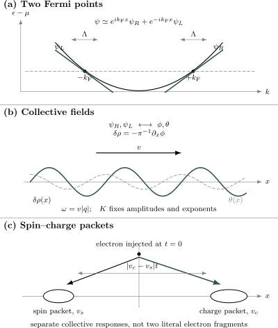
The low-energy change of variables. Near $\pm k_{\mathrm F}$, a microscopic fermion field becomes two slowly varying branches. Their density fluctuations are represented by compact fields $\phi$ and $\theta$ supporting a linearly dispersing collective mode. In a spinful liquid, one electron injection generally launches charge and spin responses with different velocities $v_c$ and $v_s$.

The Harmonic-Fluid Theory

Equations of motion

The commutator and Hamiltonian give

$$\partial_t\phi = vK\,\partial_x\theta,$$ $$\partial_t\theta = \frac vK \partial_x\phi.$$

Applying another time derivative yields

$$\left( \partial_t^2 - v^2\partial_x^2 \right) \phi = 0,$$ $$\left( \partial_t^2 - v^2\partial_x^2 \right) \theta = 0.$$

Every oscillator therefore has the linear dispersion

$$\omega(q) = v|q|.$$

Continuity equation

Using

$$\delta\rho = -\frac1\pi\partial_x\phi,$$

one finds

$$\partial_t\delta\rho = -\frac{vK}{\pi} \partial_x^2\theta.$$

With

$$j = \frac{vK}{\pi} \partial_x\theta,$$

this becomes

$$\partial_t\delta\rho + \partial_xj = 0.$$

The density mode is therefore not an analogy imposed from outside. It is the collective carrier of the conserved particle number.

Density and current stiffnesses

It is often useful to write

$$v_N = \frac vK, \qquad v_J = vK.$$

Then

$$H_{\mathrm{LL}} = \frac{\hbar}{2\pi} \int dx\, \left[ v_J(\partial_x\theta)^2 + v_N(\partial_x\phi)^2 \right].$$

The inverse relations are

$$v = \sqrt{v_Nv_J}, \qquad K = \sqrt{ \frac{v_J}{v_N} }.$$

The quantity $v_N$ measures the energy cost of changing the density, while $v_J$ measures the energy cost of a phase twist or persistent current. Their geometric mean fixes propagation; their ratio fixes the interaction-dependent scaling.

Thermodynamic and Response Meaning of the Parameters

Compressibility

For a uniform density change $\delta n$, the field has

$$\partial_x\phi = -\pi\delta n.$$

The corresponding energy density is

$$\frac{\Delta E}{L} = \frac{\pi\hbar v}{2K} (\delta n)^2.$$

Comparing with

$$\frac{\Delta E}{L} = \frac12 \frac{\partial\mu}{\partial n} (\delta n)^2$$

gives

$$\frac{\partial n}{\partial\mu} = \frac{K}{\pi\hbar v}.$$

The conventional isothermal compressibility per equilibrium density $n$ is

$$\kappa = \frac1{n^2} \frac{\partial n}{\partial\mu} = \frac{K}{\pi\hbar v n^2}.$$

These formulas apply to the single density mode in the normalization used here. Spin degeneracy or a different charge-field normalization changes prefactors.

Stiffness

A uniform phase twist has

$$\partial_x\theta = \frac{\Phi}{L}.$$

Its energy cost is

$$\Delta E = \frac{\hbar vK}{2\pi L} \Phi^2.$$

Thus a twist or Drude-weight measurement probes the product

$$vK = v_J,$$

whereas compressibility probes

$$\frac K v = \frac1{v_N}.$$

Measuring both determines $v$ and $K$ without fitting a correlation exponent.

Galilean-invariant continuum

For one spinless density mode in a Galilean-invariant continuum,

$$vK = \frac{\pi\hbar n}{m}.$$

This relation follows because a uniform phase gradient is a center-of-mass boost and the total current is tied to conserved momentum. A lattice breaks continuous Galilean invariance, so the same formula need not hold there.

Density response

For an external scalar potential coupled as

$$\delta H = \int dx\, U(x,t)\rho(x,t),$$

the retarded smooth-density susceptibility is

$$\chi_{\rho\rho}^{R}(q,\omega) = \frac{Kvq^2} {\pi\hbar \left[ (\omega+i0^+)^2-v^2q^2 \right] }.$$

The poles lie at

$$\omega = \pm v|q|.$$

The static limit is

$$\chi_{\rho\rho}^{R}(q,0) = -\frac K{\pi\hbar v}.$$

The minus sign appears because a positive external potential raises the local particle energy and reduces the density. Response to a chemical-potential perturbation has the opposite sign.

Bosonization Dictionary

Bosonization is an operator correspondence between the low-energy sectors of one-dimensional particle theories and a compact bosonic field theory. It does not claim that microscopic fermions have changed their exchange statistics.

Chiral fermion operators

For spinless fermions,

$$\begin{aligned} \psi_r(x) ={}& \frac{\eta_r}{\sqrt{2\pi a}} e^{irk_{\mathrm F}x} \\ &\times e^{-i[r\phi(x)-\theta(x)]}, \\ r ={}& \pm1. \end{aligned}$$

Here:

• $r=+1$ labels the right branch and $r=-1$ the left branch;
• $a$ is a short-distance cutoff;
• $\eta_r$ are Hermitian Klein factors;
• the vertex operator is defined with a regulator and an ordering prescription.

The Klein factors enforce anticommutation between distinct branches:

$$\{\eta_r,\eta_{r'}\} = 2\delta_{rr'}.$$

They are easy to omit in a single local correlator and essential when relative branch or species signs matter.

Density harmonics

The full long-distance density expansion is

$$\begin{aligned} \rho(x) ={}& \rho_0 - \frac1\pi\partial_x\phi(x) \\ &+ \sum_{m=1}^{\infty} A_m \cos \left( 2m[\pi\rho_0x-\phi(x)] \right). \end{aligned}$$

For spinless fermions,

$$k_{\mathrm F} = \pi\rho_0,$$

so the first oscillatory harmonic has wave number

$$2k_{\mathrm F}.$$

The smooth term is fixed by number conservation. The amplitudes $A_m$ are nonuniversal.

Bosonic particle field

For a one-dimensional bosonic fluid, the annihilation field has the asymptotic representation

$$\begin{aligned} \Psi_B(x) \sim{}& \left[ \rho_0 - \frac1\pi\partial_x\phi(x) \right]^{1/2} \\ &\times e^{+i\theta(x)} \\ &\times \sum_{m=-\infty}^{\infty} B_m e^{2im[\pi\rho_0x-\phi(x)]}. \end{aligned}$$

The creation field is the Hermitian conjugate and contains $e^{-i\theta}$. The coefficients $B_m$ depend on the cutoff and microscopic model.

Fermionic and bosonic fields differ in their allowed vertex combinations, exchange phases, and harmonic content. The quadratic Hamiltonian can nevertheless be the same.

Compactness

The density harmonics are unchanged under

$$\phi \longrightarrow \phi+\pi.$$

Particle-number quantization and boundary conditions also constrain windings of $\phi$ and $\theta$. Treating the fields as unconstrained real variables can reproduce local oscillator correlators while losing zero-mode sectors, parity rules, and the allowed operator lattice.

Vertex Operators and Scaling Dimensions

Consider

$$\mathcal O_{m,n}(x) = e^{i[m\phi(x)+n\theta(x)]}.$$

In the present normalization, its bulk scaling dimension is

$$\Delta_{m,n} = \frac14 \left( m^2K + \frac{n^2}{K} \right).$$

At equal time,

$$\left\langle \mathcal O_{m,n}(x) \mathcal O_{m,n}^{\dagger}(0) \right\rangle \propto \frac1{|x|^{2\Delta_{m,n}}}.$$

Important cases are

$$\Delta[e^{2i\phi}] = K,$$ $$\Delta[e^{2i\theta}] = \frac1K.$$

The reciprocal appearance of $K$ expresses density–phase duality: making density fluctuations costly makes phase fluctuations softer, and conversely.

The displayed dimensions assume the single-mode Hamiltonian above. Rescaling the fields changes the numerical labels $m$, $n$, and $K$ together while leaving physical exponents invariant.

Correlations in a Spinless Fermion Liquid

Density correlations

At zero temperature and distances $|x|\gg a$,

$$\begin{aligned} \left\langle \delta\rho(x) \delta\rho(0) \right\rangle \sim{}& -\frac{K}{2\pi^2x^2} \\ &+ C_1 \frac{\cos(2k_{\mathrm F}x)} {|x|^{2K}} + \cdots. \end{aligned}$$

The first term is the universal smooth-density contribution. The coefficient $C_1$ is nonuniversal, but its exponent is fixed by $K$.

Higher harmonics behave as

$$\frac{\cos(2mk_{\mathrm F}x)} {|x|^{2m^2K}}, \qquad m=2,3,\ldots.$$

One-particle correlation

The equal-time fermion correlator has

$$\left\langle \psi^\dagger(x)\psi(0) \right\rangle \sim \frac{ C_R e^{ik_{\mathrm F}x} + C_L e^{-ik_{\mathrm F}x} } {|x|^{(K+K^{-1})/2}}.$$

For a parity-symmetric state, the leading oscillation can be written as a cosine:

$$\left\langle \psi^\dagger(x)\psi(0) \right\rangle \propto \frac{\cos(k_{\mathrm F}x)} {|x|^{(K+K^{-1})/2}}.$$

The arithmetic–geometric mean inequality gives

$$\frac12 \left( K+\frac1K \right) \ge 1,$$

with equality only at

$$K=1.$$

Interactions therefore make the single-particle correlator decay faster than the free spinless-fermion result.

Density wave versus pairing

The leading $2k_{\mathrm F}$ density-wave correlation decays as

$$C_{\mathrm{CDW}}(x) \propto |x|^{-2K}.$$

A spinless pairing operator has

$$C_{\mathrm{pair}}(x) \propto |x|^{-2/K}.$$

Consequently:

• For $K<1$, density-wave correlations decay more slowly.
• For $K>1$, pair correlations decay more slowly.

These are dominant correlations, not automatically broken-symmetry order. In an ordinary short-ranged one-dimensional system, both vanish at asymptotically large separation within the gapless phase.

Correlations in a One-Dimensional Bose Liquid

The leading one-body correlation is

$$\left\langle \Psi_B^\dagger(x) \Psi_B(0) \right\rangle \propto |x|^{-1/(2K)}.$$

The leading oscillatory density term is

$$\left\langle \delta\rho(x) \delta\rho(0) \right\rangle_{2\pi\rho_0} \propto \frac{ \cos(2\pi\rho_0x) } {|x|^{2K}}.$$

For the repulsive Lieb–Liniger gas, common conventions give

$$K \ge 1.$$

The strongly repulsive Tonks–Girardeau limit approaches

$$K \longrightarrow 1,$$

while weak repulsion gives larger $K$. This does not make the weakly interacting gas a true condensate in the infinite one-dimensional thermodynamic limit; the one-body correlation remains algebraic at zero temperature.

Momentum Distribution and Vanishing Residue

Define

$$\alpha = \frac12 \left( K+\frac1K-2 \right) \ge 0.$$

Near a Fermi point, the nonanalytic part of the momentum distribution behaves schematically as

$$n(k)-n(k_{\mathrm F}) \propto -\operatorname{sgn}(k-k_{\mathrm F}) |k-k_{\mathrm F}|^{\alpha}.$$

For

$$K\ne1,$$

one has

$$\alpha>0,$$

so there is no finite jump:

$$Z = n(k_{\mathrm F}^{-}) - n(k_{\mathrm F}^{+}) = 0.$$

This is the sharpest contrast with a Landau Fermi liquid, where the jump equals the quasiparticle residue in the idealized zero-temperature translationally invariant setting.

For $\alpha>1$, analytic background terms can dominate the first derivative of $n(k)$; the power law still identifies a subleading nonanalyticity. At special integer exponents, logarithmic factors can appear. A numerical fit should therefore include regular background terms rather than forcing the entire curve into one cusp.

At the exactly free point,

$$K=1, \qquad \alpha=0,$$

and the step is restored. The limit is singular: an arbitrarily small fixed interaction produces $Z=0$ after the thermodynamic and low-energy limits are taken.

Real-Time Green Function and Spectral Thresholds

For a right mover at zero temperature, a regulated time-ordered or greater-function expression has the asymptotic structure

$$\begin{aligned} G_R(x,t) \propto{}& e^{ik_{\mathrm F}x} \left[ \frac{a} {a+i(vt-x)} \right]^{\gamma_+} \\ &\times \left[ \frac{a} {a+i(vt+x)} \right]^{\gamma_-}. \end{aligned}$$

where

$$\gamma_{\pm} = \frac14 \left( K+\frac1K\pm2 \right).$$

The exponents satisfy

$$\gamma_+ + \gamma_- = \frac12 \left( K+\frac1K \right).$$

At the free point,

$$\gamma_+ = 1, \qquad \gamma_- = 0,$$

so only the right-moving light-cone factor remains.

For $K\ne1$, both factors carry noninteger powers in general. Writing $q=k-k_{\mathrm F}$, Fourier transformation produces threshold singularities and continuum weight rather than a finite-residue Landau pole of the form

$$G^R(q,\omega) \not\sim \frac{Z} {\omega-v_{\mathrm F}q+i0^+}.$$

The local tunneling density of states of a spinless bulk liquid obeys

$$\nu_{\mathrm{bulk}}(\omega) \propto |\omega|^{\alpha}.$$

At an open end,

$$\nu_{\mathrm{end}}(\omega) \propto |\omega|^{\alpha_{\mathrm{end}}},$$

with

$$\alpha_{\mathrm{end}} = \frac1K-1$$

for the simplest spinless boundary fixed point.

Bulk and boundary exponents differ because a boundary relates right and left movers. Contacts, finite temperature, finite length, and an actual tunneling circuit can further modify the measured conductance.

The exactly linear model concentrates the smooth density response on

$$\omega = v|q|.$$

Band curvature and irrelevant interactions broaden or reshape finite-energy thresholds. The resulting nonlinear-Luttinger-liquid problem is beyond the fixed-point preview; fitting an exact delta line at nonzero experimental resolution is not a test of the asymptotic theory.

Spin–Charge Separation

Charge and spin fields

For spin-$1/2$ fermions, define

$$\phi_c = \frac{ \phi_\uparrow+\phi_\downarrow }{\sqrt2}, \qquad \phi_s = \frac{ \phi_\uparrow-\phi_\downarrow }{\sqrt2},$$

and similarly

$$\theta_c = \frac{ \theta_\uparrow+\theta_\downarrow }{\sqrt2}, \qquad \theta_s = \frac{ \theta_\uparrow-\theta_\downarrow }{\sqrt2}.$$

When symmetry allows the sectors to decouple, the fixed-point Hamiltonian is

$$H = \sum_{\nu=c,s} H_\nu,$$ $$H_\nu = \frac{\hbar v_\nu}{2\pi} \int dx\, \mathcal K_\nu(x),$$

where

$$\mathcal K_\nu = K_\nu(\partial_x\theta_\nu)^2 + \frac1{K_\nu} (\partial_x\phi_\nu)^2.$$

The charge and spin waves generally have different velocities:

$$v_c \ne v_s.$$

What an injected electron creates

An electron carries both charge and spin. Its creation operator contains vertex operators from both sectors. A localized injection therefore launches a superposition of charge and spin excitations.

After time $t$, characteristic packet centers can be separated by

$$\Delta x(t) \simeq |v_c-v_s|t.$$

This is spin–charge separation. It does not mean that the electron breaks into two microscopic fragments that can be assigned independent permanent identities. It means that charge and spin correlations propagate through distinct collective sectors.

Spin-rotation symmetry

For a gapless spin sector with exact spin-rotation invariance,

$$K_s = 1$$

at the infrared fixed point in the standard spin normalization. A marginally irrelevant spin backscattering operator can generate logarithmic corrections, so finite-size data need not look like a clean power law immediately.

Spinful exponents

With a gapless spin-rotation-invariant spin sector, the bulk tunneling exponent is

$$\alpha_{\mathrm{spinful}} = \frac14 \left( K_c+\frac1{K_c}-2 \right).$$

Representative equal-time exponents are

$$C_{2k_{\mathrm F}\mathrm{\ density}}(x) \propto |x|^{-(K_c+1)},$$ $$C_{\mathrm{singlet\ pair}}(x) \propto |x|^{-(K_c^{-1}+1)},$$

up to oscillatory factors, amplitudes, and possible logarithmic corrections.

If one sector is gapped, these formulas change. A Luther–Emery liquid, for example, has one gapless charge mode but a spin gap. Calling every spinful one-dimensional metal a two-component gapless Luttinger liquid is therefore too broad.

Central Charge and Low-Temperature Thermodynamics

Each independent nonchiral compact-boson mode has

$$c=1.$$

Thus one spinless or bosonic mode has $c=1$, gapless spin and charge modes together have $c=2$, and a spinful system with one gapped sector and one gapless sector has $c=1$ in its infrared theory.

For one mode on an infinite line, the low-temperature free-energy density is

$$f(T) = e_0 - \frac{\pi c}{6} \frac{(k_{\mathrm B}T)^2} {\hbar v} + o(T^2).$$

The specific heat per length is

$$\frac{C_V}{L} = \frac{\pi c}{3} \frac{k_{\mathrm B}^2T} {\hbar v} + o(T).$$

For several decoupled modes,

$$\frac{C_V}{L} = \frac{\pi k_{\mathrm B}^2T}{3\hbar} \sum_\nu \frac{c_\nu}{v_\nu} + o(T).$$

A linear heat capacity alone does not uniquely identify a Luttinger liquid, but its coefficient provides a stringent consistency test when $v$ is known independently.

Finite Temperature

Define the thermal length scale

$$\ell_T = \frac{\hbar v} {\pi k_{\mathrm B}T}.$$

For an operator of scaling dimension $\Delta$, the zero-temperature power law maps to

$$\left( \frac a{|x|} \right)^{2\Delta} \longrightarrow \left[ \frac{ \pi a k_{\mathrm B}T/(\hbar v) } { \sinh( \pi k_{\mathrm B}T|x|/(\hbar v) ) } \right]^{2\Delta}.$$

At short separation,

$$|x| \ll \ell_T,$$

the zero-temperature power law is recovered. At long separation,

$$|x| \gg \ell_T,$$

the same correlator decays exponentially:

$$C_{\mathcal O}(x,T) \propto \exp \left[ -\frac{ 2\pi\Delta k_{\mathrm B}T }{\hbar v} |x| \right].$$

Different operators have different $\Delta$, so there is no unique correlation length shared by every observable. The scale $\ell_T$ marks the common quantum-to-thermal crossover.

For spin and charge sectors with different velocities, each factor carries its own thermal length:

$$\ell_{T,\nu} = \frac{\hbar v_\nu} {\pi k_{\mathrm B}T}.$$

Finite Size and Zero Modes

Ground-state Casimir term

For one periodic gapless mode on a ring of circumference $L$,

$$E_0(L) = Le_\infty - \frac{\pi\hbar vc}{6L} + o(L^{-1}).$$

The coefficient of the $1/L$ term contains the universal central charge, but extracting it requires an independently known velocity and control of subleading corrections.

For an open chain, the boundary condition changes the coefficient. One must not fit periodic data with the open-chain formula or conversely.

Number and current sectors

Let $\Delta N$ be the particle-number change relative to a reference sector and let $J$ be the winding or current quantum number. A common periodic-ring spectrum is

$$\begin{aligned} \Delta E ={}& \frac{\pi\hbar v}{2L} \left[ \frac{(\Delta N)^2}{K} + KJ^2 \right] \\ &+ \frac{2\pi\hbar v}{L} \left( N_R+N_L \right). \end{aligned}$$

The nonnegative integers $N_R$ and $N_L$ count total right- and left-moving oscillator levels. This formula displays three distinct probes:

$$\begin{array}{c|c} \text{number change} & v/K \\[3pt] \text{current or twist} & vK \\[3pt] \text{oscillator spacing} & v \end{array}$$

The allowed combinations of $\Delta N$ and $J$ depend on statistics, microscopic filling, boundary conditions, and parity sector. The quadratic energy is universal; the selection rules are part of the compactification data and must be matched to the microscopic model.

Entanglement check

A periodic $c=1$ liquid has interval entropy

$$S(\ell,L) = \frac13 \ln \left[ \frac{L}{\pi a} \sin \left( \frac{\pi\ell}{L} \right) \right] + s_1$$

at leading order. This is a valuable central-charge diagnostic, but oscillatory and marginal corrections can bias short-chain fits. Entanglement Entropy owns the boundary variants, Rényi formulas, fitting cautions, and area-law comparison.

Perturbations Around the Fixed Line

The Luttinger Hamiltonian is a fixed-point theory. Microscopic symmetries determine which additional operators are allowed. Their scaling dimensions determine whether they fade, remain marginal, or grow under coarse-graining.

Bulk cosine

Consider

$$\delta H_p = g_p \int dx\, \cos(2p\phi).$$

Its bulk scaling dimension is

$$\Delta_p = p^2K.$$

To leading order, the dimensionless coupling obeys

$$\frac{dg_p}{d\ell} = \left( 2-p^2K \right)g_p + \cdots.$$

Therefore:

$$\begin{array}{c|c} p^2K<2 & \text{relevant} \\[3pt] p^2K>2 & \text{irrelevant} \\[3pt] p^2K=2 & \text{marginal at tree level} \end{array}$$

At marginality, higher-order flow decides the outcome. A relevant cosine can pin $\phi$ near one of its minima and gap the corresponding density sector.

Spinless half-filled Umklapp

For a translation-invariant spinless lattice at half filling, the leading allowed Umklapp term has

$$\delta H_{\mathrm U} \propto \int dx\, \cos(4\phi).$$

Its dimension is

$$\Delta_{\mathrm U} = 4K.$$

It becomes relevant when

$$K < \frac12.$$

The equality marks the Berezinskii–Kosterlitz–Thouless threshold in the standard short-ranged problem. Spinless Fermion Chains owns how this criterion appears in the $t$–$V$ phase diagram.

Commensurate bosons

For bosons at the simplest integer commensurability in a periodic lattice, the leading pinning term is commonly

$$\delta H_{\mathrm{lat}} \propto \int dx\, \cos(2\phi).$$

Its dimension is

$$\Delta_{\mathrm{lat}} = K,$$

so the corresponding BKT threshold occurs at

$$K=2$$

in this normalization. Different commensurabilities produce higher harmonics and different thresholds.

Pairing perturbation

If particle-number conservation is explicitly broken, for example by proximity coupling, a spinless pairing perturbation can contain

$$\delta H_{\mathrm{pair}} \propto \int dx\, \cos(2\theta).$$

Its dimension is

$$\Delta_{\mathrm{pair}} = \frac1K.$$

It is relevant at tree level when

$$K > \frac12.$$

The density-pinning and phase-pinning cosines are dual competitors. They cannot both be treated as simultaneously sharp classical fields because $\phi$ and $\theta$ are conjugate.

Single impurity

A local backscattering impurity at $x=0$ produces

$$\delta H_{\mathrm{imp}} = \lambda \cos[2\phi(0)].$$

As a boundary operator, it has dimension

$$\Delta_{\mathrm{imp}} = K.$$

Its leading flow is

$$\frac{d\lambda}{d\ell} = (1-K)\lambda + \cdots.$$

Thus a weak impurity grows for repulsive spinless liquids with $K<1$. The dual weak-link amplitude $t_{\mathrm{link}}$ has boundary dimension

$$\Delta_{\mathrm{link}} = \frac1K$$

and flow

$$\frac{dt_{\mathrm{link}}}{d\ell} = \left( 1-\frac1K \right)t_{\mathrm{link}} + \cdots.$$

This weak-barrier/weak-link duality describes the asymptotic isolated Luttinger liquid. Leads, finite length, multiple channels, resonant levels, and additional symmetries can change the measured transport crossover.

Spin and charge gaps

In a spinful system, backscattering can generate a cosine in the spin sector, while commensurate Umklapp can generate one in the charge sector. Depending on its sign and scaling flow, a cosine may:

• remain marginally irrelevant and leave the sector gapless;
• become relevant and pin the field;
• produce a spin gap with gapless charge;
• produce a charge gap with gapless or gapped spin;
• leave two gapless sectors.

The phrase “Luttinger liquid” should therefore be accompanied by the number and identity of the gapless modes.

Representative Microscopic Realizations

Repulsive contact bosons

The Lieb–Liniger Model Preview is the canonical finite-coupling dossier for continuum bosons with repulsive delta-function interactions. Its low-energy phase is a one-mode Luttinger liquid throughout the repulsive regime. Exact Bethe-ansatz thermodynamics determines $v$ and $K$, while the universal page here determines how those values enter long-distance observables.

Spinless lattice fermions

The half-filled $t$–$V$ chain is a Luttinger liquid between phase separation and charge-density-wave order. Its free point has $K=1$; repulsion lowers $K$, and the commensurate charge-order threshold is reached at $K=1/2$.

XXZ spin chain

The easy-plane spin-$1/2$ XXZ chain has one gapless compact-boson mode. Spin operators map to uniform and staggered vertex operators. The exactly known dependence of $K$ and $v$ on anisotropy belongs to XXZ Spin Chain.

One-dimensional Bose–Hubbard superfluid

The compressible side of the one-dimensional Bose–Hubbard model is described by a Luttinger liquid. At commensurate filling, a lattice cosine can become relevant and drive a Mott transition. The universal threshold is stated above; Bose–Hubbard Chain owns the microscopic one-dimensional Hamiltonian, exact limits, numerical transition scale, and finite-size diagnostics, while the general lattice treatment remains at Bose–Hubbard Model.

Repulsive Hubbard chain away from commensurability

Away from a charge-gapping commensurability, the repulsive one-dimensional Hubbard model has separate gapless charge and spin sectors. Spin-rotation symmetry fixes the infrared spin normalization, while interactions renormalize the charge parameter and separate the velocities.

Quantum wires and cold-atom tubes

Semiconductor wires, carbon nanotubes, atomic gases confined to tubes, and chains in crystalline solids can display Luttinger-liquid scaling over a finite window. Real samples also contain contacts, transverse modes, disorder, long-range Coulomb interactions, and finite temperature. Demonstrating the fixed point requires showing a common parameter set across several observables, not merely fitting one power law.

How to Extract the Luttinger Data

Small-momentum structure factor

Define the equal-time continuum structure factor per length by

$$s(q) = \frac1L \left\langle \delta\rho_q \delta\rho_{-q} \right\rangle,$$

with

$$\delta\rho_q = \int_0^L dx\, e^{-iqx}\delta\rho(x).$$

The fixed point predicts

$$s(q) = \frac{K|q|}{2\pi} + o(|q|).$$

Hence

$$K = 2\pi \lim_{q\to0} \frac{s(q)}{|q|}.$$

On a lattice, the definition of density per site and the Fourier normalization must be translated before applying this prefactor.

Compressibility and stiffness

The two independent combinations are

$$\frac K v = \pi\hbar \frac{\partial n}{\partial\mu},$$ $$vK = v_J.$$

Their product and ratio give

$$K = \sqrt{ \left( \pi\hbar \frac{\partial n}{\partial\mu} \right) v_J },$$ $$v = \sqrt{ \frac{ v_J }{ \pi\hbar \partial n/\partial\mu } }.$$

The dimensions of $v_J$ depend on the stiffness convention. The equations above assume it has velocity units as in the Hamiltonian ledger.

Finite-size levels

The oscillator spacing gives

$$\Delta E_{\mathrm{osc}} \simeq \frac{2\pi\hbar v}{L}.$$

Number and winding gaps then separate $v/K$ and $vK$. This method is powerful in exact diagonalization and density-matrix renormalization group calculations, provided the correct symmetry and parity sectors are identified.

Correlation exponents

One can fit several predictions:

$$\eta_{2k_{\mathrm F}} = 2K,$$ $$\eta_{\mathrm{pair}} = \frac2K,$$ $$\eta_{\mathrm{fermion}} = \frac12 \left( K+\frac1K \right).$$

A reliable identification asks whether one value of $K$ explains all accessible exponents after finite-size, boundary, temperature, and logarithmic corrections are included.

Velocity-resolved response

The slope of a low-$q$ density mode gives $v$. In a spinful system, charge- and spin-sensitive probes can reveal separate slopes:

$$\omega_c(q) \simeq v_c|q|,$$ $$\omega_s(q) \simeq v_s|q|.$$

Spectral continua and matrix elements can obscure a simple line, so one should track thresholds and integrated response rather than only the brightest pixel.

Central charge

Finite-size ground-state energies and entanglement scaling can test

$$c=1$$

per gapless nonchiral mode. Central charge counts modes; it does not determine $K$. Two $c=1$ liquids can have different exponents.

A Consistency Workflow

1. Identify the active dimension. Verify that transverse excitation, temperature, drive, and interaction scales lie below the confinement gap.
2. Count gapless sectors. Determine whether charge, spin, flavor, or band modes remain gapless.
3. State the field normalization. Record the commutator, density map, and Hamiltonian before quoting $K$.
4. Determine the infrared window. Exclude distances comparable to the cutoff, the system size, and the thermal length.
5. Extract $v$ independently. Use a mode slope or finite-size oscillator gap.
6. Extract $K$ in more than one way. Compare structure factor, compressibility and stiffness, and correlation exponents.
7. Test perturbations. Check commensurability, impurities, disorder, pairing, and spin backscattering.
8. Inspect single-particle evidence. Look for a cusp and threshold continuum rather than assuming a Lorentzian pole.
9. Control corrections. Vary size, temperature, fit window, broadening, and boundary conditions.
10. Report the regime. State the energy, momentum, length, and temperature window over which the Luttinger description is supported.

Where the Linear Theory Stops

Band curvature

The exact microscopic dispersion is not linear:

$$\epsilon(k) -\mu = \hbar v_{\mathrm F}\delta k + \frac{\hbar^2}{2m_*} (\delta k)^2 + \cdots.$$

Curvature is irrelevant in the strict fixed-point sense but reorganizes finite-energy threshold singularities. It can determine decay channels, line shapes, and asymmetry near spectral edges.

Gapped phases

If a relevant cosine pins a field, the asymptotic theory is no longer the gapless Gaussian Hamiltonian. Correlations of some operators become exponential, solitons or massive particles can replace the sound mode, and the $c=1$ finite-size formulas cease to apply below the gap.

Long-range interactions

Unscreened or weakly screened Coulomb interactions can make the effective parameters momentum dependent:

$$K \longrightarrow K(q), \qquad v \longrightarrow v(q).$$

The resulting correlations need not be simple powers with one constant exponent. Calling such a system an ordinary short-ranged Luttinger liquid can hide physically important logarithms.

Disorder

Random backscattering introduces a spatially varying operator rather than one isolated boundary impurity. Its relevance criterion and localized phase are not obtained by applying the single-impurity result point by point. Renormalization Group Preview owns the general flow logic; disorder-specific flows require their own treatment.

Multiple channels

Two bands, valleys, legs, or internal components produce a matrix of density and phase couplings. Diagonalization may yield several collective modes with different velocities and compactification data. A single pair $(v,K)$ is then insufficient.

Boundaries and leads

An open boundary folds right movers into left movers and changes local exponents. A clean interacting wire connected adiabatically to noninteracting reservoirs can have a two-terminal conductance governed by the leads even though its local tunneling density of states shows interaction-dependent powers.

Dimensional crossover

Interchain hopping or transverse excitation can become relevant at sufficiently low energy. A material may show Luttinger scaling over an intermediate window and cross over to higher-dimensional coherent motion, ordering, or Fermi-liquid behavior at longer scales.

Chiral edge liquids

A fractional quantum Hall edge can be described by a chiral Luttinger theory. Its anomaly, compactification, charge assignments, and one-way propagation differ from the nonchiral right-plus-left liquid developed here. The shared word “Luttinger” does not make the two theories interchangeable.

Integrability

Integrability is not required for Luttinger-liquid universality. It is one way to calculate $v$, $K$, and exact crossover functions in special microscopic models. Generic nonintegrable short-ranged systems can flow to the same fixed point.

Common Mistakes

Treating the Luttinger parameter as self-defining

A quoted value of $K$ is incomplete without the field normalization, species convention, and operator dictionary. Spin-chain, spinful-charge, and bosonic conventions can differ by factors of two.

Calling every one-dimensional system a Luttinger liquid

One-dimensional systems can be gapped, localized, phase separated, symmetry broken, topological, many-channel, or governed by long-range interactions. The label requires a gapless compact-boson sector and a demonstrated infrared window.

Interpreting bosonization literally

Bosonization rewrites low-energy operators. It does not turn a microscopic fermion into a microscopic boson or erase anticommutation. Klein factors and compactification retain the statistics and global sectors.

Looking for a narrow Landau peak

The generic single-particle signal is threshold continuum weight with no finite residue. A narrow finite-size or resolution-broadened feature is not by itself a quasiparticle pole.

Calling dominant correlations long-range order

The slowest algebraic decay identifies the leading susceptibility, not a nonzero infinite-distance order parameter.

Confusing spin–charge separation with fractional particles

Different collective sectors carry the response at different velocities. This operational statement is subtler than a picture of one electron permanently breaking into two localized pieces.

Ignoring the order of limits

For a weak but fixed interaction,

$$Z=0$$

in the thermodynamic infrared limit. A short finite system can retain an apparently sharp overlap because the flow is cut off before the asymptotic regime is reached.

Fitting one power law over one decade

Crossovers, boundaries, thermal decay, marginal logarithms, and analytic backgrounds can all imitate an exponent. A trustworthy claim combines several observables and varies the fit window.

Worked Checks

Recover the free spinless point

Set

$$K=1, \qquad v=v_{\mathrm F}.$$

Then

$$\gamma_+ = 1, \qquad \gamma_- = 0,$$

and

$$\alpha = 0.$$

The right-moving Green function reduces to one chiral denominator, the momentum distribution regains a jump, and the density and pairing exponents are both $2$. The fixed-point Hamiltonian therefore contains the free gas as one special point, not as a separate formalism.

A repulsive example

Take a spinless liquid with

$$K = \frac34.$$

The leading density-wave exponent is

$$\eta_{\mathrm{CDW}} = 2K = \frac32,$$

while the pairing exponent is

$$\eta_{\mathrm{pair}} = \frac2K = \frac83.$$

Density correlations decay more slowly. The momentum cusp exponent is

$$\alpha = \frac12 \left( \frac34 + \frac43 - 2 \right) = \frac1{24}.$$

The exponent is small, so a finite system may look almost discontinuous even though the true thermodynamic jump is zero.

Reconstruct the velocity and Luttinger parameter

Suppose finite-size energies yield

$$v_N = 1.8u, \qquad v_J = 0.8u,$$

where $u$ is a velocity unit. Then

$$v = \sqrt{1.44}\,u = 1.2u,$$

and

$$K = \sqrt{ \frac{0.8}{1.8} } = \frac23.$$

The inferred $K<1$ is consistent with repulsive spinless behavior. The conclusion is stronger if the $2k_{\mathrm F}$ density exponent also approaches

$$2K = \frac43.$$

Exercises

Exercise 1: Wave equation and continuity

Starting from

$$\partial_t\phi = vK\partial_x\theta, \qquad \partial_t\theta = \frac vK\partial_x\phi,$$

derive the wave equation for $\phi$. Then use the density definition to identify the conserved current.

Solution

Differentiate the first equation with respect to time:

$$\partial_t^2\phi = vK \partial_x\partial_t\theta.$$

Insert the second equation:

$$\partial_t^2\phi = vK \partial_x \left( \frac vK \partial_x\phi \right) = v^2\partial_x^2\phi.$$

Therefore

$$\left( \partial_t^2-v^2\partial_x^2 \right)\phi = 0.$$

Since

$$\delta\rho = -\frac1\pi\partial_x\phi,$$

one has

$$\partial_t\delta\rho = -\frac{vK}{\pi} \partial_x^2\theta.$$

Writing this as

$$\partial_t\delta\rho + \partial_xj = 0$$

identifies

$$j = \frac{vK}{\pi} \partial_x\theta.$$

Exercise 2: Density and current velocities

A finite-size calculation gives

$$v_N = 3u, \qquad v_J = u.$$

Find $v$ and $K$. Which qualitative spinless interaction regime does the value of $K$ suggest?

Solution

The collective velocity is

$$v = \sqrt{v_Nv_J} = \sqrt3\,u.$$

The Luttinger parameter is

$$K = \sqrt{ \frac{v_J}{v_N} } = \frac1{\sqrt3}.$$

Because

$$K<1,$$

the result is characteristic of repulsive spinless interactions in this normalization. That inference can fail if the field or species convention differs, so the Hamiltonian normalization must accompany the quoted number.

Exercise 3: Free limit of the chiral correlator

Evaluate $\gamma_+$, $\gamma_-$, and $\alpha$ at $K=1$. Explain what happens to the counterpropagating factor in $G_R(x,t)$.

Solution

At $K=1$,

$$\gamma_{\pm} = \frac14 (1+1\pm2).$$

Therefore

$$\gamma_+ = 1, \qquad \gamma_- = 0.$$

The factor involving $vt+x$ is raised to the zeroth power and disappears. The right-moving correlator becomes

$$G_R(x,t) \propto e^{ik_{\mathrm F}x} \frac a{a+i(v_{\mathrm F}t-x)}.$$

Also,

$$\alpha = \frac12(1+1-2) = 0,$$

consistent with the free momentum-distribution step.

Exercise 4: A cusp without a jump

For a spinless liquid with $K=1/2$, compute the momentum-distribution exponent. Does $n(k)$ have a jump at $k_{\mathrm F}$?

Solution

The exponent is

$$\alpha = \frac12 \left( \frac12 + 2 - 2 \right) = \frac14.$$

Near the Fermi point,

$$\begin{aligned} n(k)-n(k_{\mathrm F}) \propto{}& -\operatorname{sgn}(k-k_{\mathrm F}) \\ &\times |k-k_{\mathrm F}|^{1/4}. \end{aligned}$$

The function is continuous, although its slope is singular. Hence

$$Z=0.$$

Exercise 5: Competing correlations

For $K=3/4$, compare the leading spinless density-wave and pairing exponents. Which correlation decays more slowly?

Solution

The density-wave exponent is

$$\eta_{\mathrm{CDW}} = 2K = \frac32.$$

The pairing exponent is

$$\eta_{\mathrm{pair}} = \frac2K = \frac83.$$

Because

$$\frac32 < \frac83,$$

the $2k_{\mathrm F}$ density correlation decays more slowly. This identifies the dominant algebraic tendency, not true charge-density-wave long-range order.

Exercise 6: Arrival-time separation

A probe injects an electron a distance $d$ from a detector. The charge and spin velocities are $v_c$ and $v_s$, with $v_c>v_s>0$. Find the separation between the arrival times. What does the detector observe if its time resolution is worse than this separation?

Solution

The characteristic arrival times are

$$t_c = \frac d{v_c}, \qquad t_s = \frac d{v_s}.$$

Their separation is

$$\Delta t = t_s-t_c = d \left( \frac1{v_s} - \frac1{v_c} \right).$$

If the instrumental time resolution exceeds $\Delta t$, the two responses overlap and may appear as one broadened pulse. Failure to resolve two peaks is then not evidence that $v_c=v_s$.

Exercise 7: Classify four perturbations

At a spinless fixed point with

$$K=0.4,$$

classify the following at tree level:

1. half-filled Umklapp $\cos(4\phi)$;
2. a local impurity $\cos[2\phi(0)]$;
3. a weak link;
4. a bulk pairing term $\cos(2\theta)$.

Solution

The half-filled Umklapp dimension is

$$\Delta_{\mathrm U} = 4K = 1.6.$$

Because this is a bulk operator and

$$1.6<2,$$

it is relevant.

The local impurity has boundary dimension

$$\Delta_{\mathrm{imp}} = K = 0.4<1,$$

so it is relevant.

The weak link has boundary dimension

$$\Delta_{\mathrm{link}} = \frac1K = 2.5>1,$$

so it is irrelevant near the cut-chain fixed point.

The bulk pairing cosine also has dimension

$$\Delta_{\mathrm{pair}} = \frac1K = 2.5>2,$$

so it is irrelevant at tree level.

The comparison threshold is $2$ for bulk operators and $1$ for boundary operators.

Exercise 8: Finite-size spectroscopy

For a periodic one-mode liquid, compare the lowest energy costs of the sectors

$$(\Delta N,J)=(1,0)$$

and

$$(\Delta N,J)=(0,1),$$

ignoring oscillator excitations. Show how their ratio determines $K$.

Solution

The number-changing gap is

$$\Delta E_N = \frac{\pi\hbar v}{2LK}.$$

The winding gap is

$$\Delta E_J = \frac{\pi\hbar vK}{2L}.$$

Their ratio is

$$\frac{\Delta E_J}{\Delta E_N} = K^2.$$

Therefore

$$K = \sqrt{ \frac{\Delta E_J}{\Delta E_N} }.$$

In a microscopic fermion problem, the sectors $(1,0)$ and $(0,1)$ may not both satisfy the parity selection rule. One must use the lowest allowed sectors and adjust the integer changes accordingly.

Key Takeaways

• A Luttinger liquid replaces particle-like low-energy excitations by collective density and phase waves.
• One gapless mode is controlled by a velocity $v$ and a convention-dependent parameter $K$.
• The same $K$ fixes compressibility, stiffness ratios, density harmonics, pairing powers, tunneling suppression, and the momentum cusp.
• A generic interacting spinless liquid has $Z=0$ even when the interaction is arbitrarily weak.
• Spinful systems can separate into charge and spin sectors with different velocities.
• Relevant commensurate, impurity, pairing, spin, or disorder perturbations can drive the system away from the gapless fixed line.
• Central charge counts gapless modes, while $K$ distinguishes points along a fixed line.
• Trustworthy identification requires one parameter set to explain several observables over a controlled infrared window.

Cross-Links

• Quantum Wires for the material realization, transverse subbands, threshold density of states, and evidence boundary between one-particle mode structure and Luttinger-liquid behavior.
• Low-Dimensional Quantum Gases for confinement criteria, one-dimensional kinematics, and infrared fluctuation constraints.
• Fermi Liquid Theory Preview for the finite-residue quasiparticle framework that Luttinger liquids replace.
• Fractionalization for the cross-dimensional physical criteria and evidence boundary beyond the canonical one-dimensional field theory developed here.
• Collective Modes for response poles, damping, and general mode language.
• Perturbation Theory in Many-Body Systems for why fixed-order expansions can fail in the one-dimensional infrared.
• Spinless Fermion Chains for the $t$–$V$ model and exact Luttinger data.
• XXZ Chain dossier for the convention-complete microscopic record and exact zero-field Luttinger parameters.
• XXZ Spin Chain for a spin realization with a $c=1$ critical interval.
• Renormalization Group Preview for fixed lines, scaling dimensions, relevance, and crossover.
• Spectral Functions for spectral normalization, thresholds, broadening, and experimental intensity.
• Entanglement Entropy for central-charge extraction and finite-size fitting.
• Entanglement and Criticality for the $c=1$ fixed-line signature, chord-length fits, and finite-entanglement scaling.
• Why Many-Body QM Leads to QFT for the broader operator-field-theory bridge.
• Condensed Matter Roadmap for a study sequence through quantum matter.
• Bridge to QFT Roadmap for the continuation from many-body bosonization to field theory.

References

1. S. Tomonaga, “Remarks on Bloch’s Method of Sound Waves Applied to Many-Fermion Problems”, Progress of Theoretical Physics 5, 544–569 (1950).
2. J. M. Luttinger, “An Exactly Soluble Model of a Many-Fermion System”, Journal of Mathematical Physics 4, 1154–1162 (1963).
3. D. C. Mattis and E. H. Lieb, “Exact Solution of a Many-Fermion System and Its Associated Boson Field”, Journal of Mathematical Physics 6, 304–312 (1965).
4. F. D. M. Haldane, “‘Luttinger Liquid Theory’ of One-Dimensional Quantum Fluids. I”, Journal of Physics C 14, 2585–2609 (1981).
5. A. Luther and I. Peschel, “Calculation of Critical Exponents in Two Dimensions from Quantum Field Theory in One Dimension”, Physical Review B 12, 3908–3917 (1975).
6. J. Voit, “One-Dimensional Fermi Liquids”, Reports on Progress in Physics 58, 977–1116 (1995).
7. T. Giamarchi, Quantum Physics in One Dimension, Oxford University Press (2004).
8. J. von Delft and H. Schoeller, “Bosonization for Beginners — Refermionization for Experts”, Annalen der Physik 7, 225–305 (1998).
9. M. A. Cazalilla, “Bosonizing One-Dimensional Cold Atomic Gases”, Journal of Physics B 37, S1–S47 (2004).
10. M. A. Cazalilla, R. Citro, T. Giamarchi, E. Orignac, and M. Rigol, “One Dimensional Bosons: From Condensed Matter Systems to Ultracold Gases”, Reviews of Modern Physics 83, 1405–1466 (2011).
11. E. H. Lieb and W. Liniger, “Exact Analysis of an Interacting Bose Gas. I. The General Solution and the Ground State”, Physical Review 130, 1605–1616 (1963).
12. E. H. Lieb and F. Y. Wu, “Absence of Mott Transition in an Exact Solution of the Short-Range, One-Band Model in One Dimension”, Physical Review Letters 20, 1445–1448 (1968).
13. A. Luther and V. J. Emery, “Backward Scattering in the One-Dimensional Electron Gas”, Physical Review Letters 33, 589–592 (1974).
14. C. L. Kane and M. P. A. Fisher, “Transport in a One-Channel Luttinger Liquid”, Physical Review Letters 68, 1220–1223 (1992).
15. T. Giamarchi and H. J. Schulz, “Anderson Localization and Interactions in One-Dimensional Metals”, Physical Review B 37, 325–340 (1988).
16. A. Imambekov, T. L. Schmidt, and L. I. Glazman, “One-Dimensional Quantum Liquids: Beyond the Luttinger Liquid Paradigm”, Reviews of Modern Physics 84, 1253–1306 (2012).
17. Y. Jompol et al., “Probing Spin-Charge Separation in a Tomonaga–Luttinger Liquid”, Science 325, 597–601 (2009).