Why Many-Body QM Leads to QFT

Many-body quantum mechanics makes field theory natural because its important questions are usually about modes, local densities, correlations, collective behavior, and scale dependence, not the trajectories or labels of individual particles. A field operator packages infinitely many position-space modes into one local object. A collective field packages the long-wavelength behavior of many microscopic degrees of freedom. Correlation functions then become the primary bridge between theory and observable response.

This progression does not mean that every many-body problem becomes a relativistic quantum field theory. It means that the language and methods of fields become more economical than a fixed-$N$ wavefunction description:

$$\begin{gathered} \text{particle coordinates} \longrightarrow \text{mode occupations} \longrightarrow \text{local operator fields}, \\ \text{local operator fields} \longrightarrow \text{correlators and collective fields} \longrightarrow \text{effective field theory}. \end{gathered}$$

Relativistic QFT adds essential principles, including Lorentz symmetry and spacetime locality, that do not follow from nonrelativistic many-body mechanics alone.

Canonical Scope

This page is the conceptual bridge from many-body quantum mechanics to field-theoretic thinking. It owns:

• why labeled-particle wavefunctions become an awkward organizing language;
• how Fock space and local fields reorganize the same many-particle physics;
• why correlation functions and sources become central;
• how order parameters, auxiliary fields, and collective modes differ from microscopic particle fields;
• how finite temperature, imaginary time, and coarse-graining lead toward statistical field theory;
• the distinction between nonrelativistic field theory, emergent effective field theory, and relativistic QFT;
• a route map showing where each technical construction continues.

It does not repeat neighboring derivations:

• Occupation-Number Representation owns many-body Fock-space bookkeeping.
• Field Operators in Many-Body Models owns explicit nonrelativistic Hamiltonians and their operator algebra.
• Second Quantization: Bridge to QFT owns the general Fock-space handoff from composite-system quantum mechanics.
• Correlation Functions Overview and Kubo Formula own many-body correlators and linear response.
• Dynamics: Bridge to QFT owns the detailed path from evolution operators, propagators, sources, and path integrals to QFT observables.
• Bridge to QFT Roadmap owns the site-wide learning sequence.

Three Meanings of Field Language

The word “field” appears in several related but distinct senses.

Field object	Typical example	Status
microscopic operator field	$\psi(\mathbf x)$ for atoms or electrons	exact rewriting of a many-particle model
auxiliary field	Hubbard–Stratonovich density or pairing field	exact transformation only when the functional identity and contour are specified
collective or order-parameter field	magnetization $\phi(\mathbf x,\tau)$ or condensate amplitude $\Phi(\mathbf x,\tau)$	coarse-grained or expectation-value description
quasiparticle field	low-energy fermion, phonon, or magnon field	effective description within a scale window
relativistic quantum field	scalar, spinor, or gauge field on spacetime	local quantum framework constrained by relativistic symmetry

These objects can be connected, but they should not be identified without an argument. A microscopic annihilation operator, an auxiliary integration variable, and a coarse-grained order parameter can obey different algebras and have different domains of validity.

Why Fixed-Particle Coordinates Become Awkward

For $N$ distinguishable particles, a wavefunction has the form

$$\Psi_N(x_1,\ldots,x_N),$$

where each $x_i$ may include position and internal labels. Identical particles require

$$\Psi_N(\ldots,x_i,\ldots,x_j,\ldots) = \eta\, \Psi_N(\ldots,x_j,\ldots,x_i,\ldots),$$

with

$$\eta = \begin{cases} +1, & \text{bosons},\\ -1, & \text{fermions}. \end{cases}$$

This representation is exact, but several difficulties grow with $N$:

• permutation symmetry is built into a function of many redundant labels;
• adding or removing a particle changes the number of arguments;
• observables such as density and current require sums over all particle coordinates;
• the thermodynamic limit changes the very dimension of configuration space;
• collective excitations are distributed across many coordinates;
• locality is less transparent than in a position-space operator language.

The problem is not that first quantization becomes wrong. It is that its coordinates no longer match the objects one wants to manipulate.

From Particles to Modes

Choose one-particle modes $\{\varphi_i\}$ and record how many particles occupy each mode:

$$\lvert n_1,n_2,\ldots\rangle.$$

The bosonic or fermionic Fock space is a direct sum of fixed-number sectors,

$$\mathcal F_\eta(\mathcal h) = \bigoplus_{N=0}^{\infty} \mathcal H_N^{(\eta)}.$$

The total number operator is

$$\widehat N = \sum_i a_i^\dagger a_i.$$

Creation and annihilation operators connect neighboring sectors:

$$\begin{aligned} a_i^\dagger &: \mathcal H_N^{(\eta)} \longrightarrow \mathcal H_{N+1}^{(\eta)}, \\ a_i &: \mathcal H_N^{(\eta)} \longrightarrow \mathcal H_{N-1}^{(\eta)}. \end{aligned}$$

Their commutators with total number make that meaning precise:

$$[\widehat N,a_i^\dagger] = a_i^\dagger, \qquad [\widehat N,a_i] = -a_i.$$

Fock space allows variable particle number, but it does not require number-changing dynamics. If

$$[H,\widehat N]=0,$$

then every fixed-$N$ sector evolves independently. The grand-canonical operator

$$K = H-\mu\widehat N$$

weights sectors differently in an ensemble; it does not by itself violate particle-number conservation.

From Modes to Local Operator Fields

A position-space annihilation field is a mode expansion,

$$\psi(x) = \sum_i \varphi_i(x)a_i,$$

with

$$\psi^\dagger(x) = \sum_i \varphi_i^*(x)a_i^\dagger.$$

For a complete orthonormal basis, the mode algebra implies the equal-time field algebra

$$\begin{aligned} [\psi(x),\psi^\dagger(y)] &= \delta(x-y) \qquad \text{for bosons}, \\ \{\psi(x),\psi^\dagger(y)\} &= \delta(x-y) \qquad \text{for fermions}. \end{aligned}$$

The local number density is

$$n(x) = \psi^\dagger(x)\psi(x),$$

and the total number is

$$\widehat N = \int dx\, n(x).$$

The position label is now attached to an operator, not to a permanently labeled particle. The field removes an excitation from a localized one-particle mode, while the many-body state records all occupations and correlations.

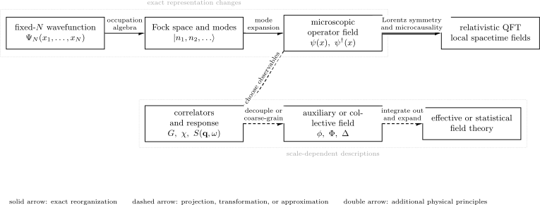
Field language enters in more than one way. Mode and operator fields can exactly reorganize a nonrelativistic many-particle theory. Collective fields arise after choosing observables and scales. Relativistic QFT adds spacetime symmetry and locality rather than following from a change of notation alone.

Exact Rewriting Within a Fixed Sector

Consider a nonrelativistic $N$-particle Hamiltonian

$$H_N = \sum_{i=1}^{N} h(x_i) + \frac12 \sum_{i\ne j} V(x_i,x_j).$$

Its field-operator form is

$$\begin{aligned} H &= \int dx\, \psi^\dagger(x) h \psi(x) \\ &\quad + \frac12 \int dx\,dy\, \psi^\dagger(x) \psi^\dagger(y) V(x,y) \psi(y) \psi(x). \end{aligned}$$

Restricted to the $N$-particle sector, this operator reproduces the first-quantized Hamiltonian with the correct Bose or Fermi exchange symmetry. No new physics has been introduced merely by changing representation.

This equivalence has conditions:

• the one-particle space and particle species are fixed;
• the domains and boundary conditions match;
• continuum products are regulated when necessary;
• the interaction and operator ordering use consistent conventions;
• the comparison is made in the same number sector.

The full derivation and regularization cautions belong to Field Operators in Many-Body Models.

Why the Field Form Is More Than Cosmetic

An exact change of representation can still expose new structure.

Locality

A short-range Hamiltonian becomes an integral or sum of local operator products. Continuity equations, conserved currents, boundary terms, and response to local sources become easier to state.

Symmetry

A global $U(1)$ transformation acts locally on the field:

$$\psi(x) \longmapsto e^{i\alpha}\psi(x).$$

Its generator is $\widehat N$. Continuous spatial symmetries, internal rotations, and gauge couplings likewise act directly on fields and their derivatives.

Correlations

The one-body density matrix is a two-point function,

$$G^{(1)}(x,y) = \langle \psi^\dagger(x)\psi(y) \rangle.$$

Density correlations are field correlators,

$$C_{nn}(x,y) = \langle n(x)n(y)\rangle - \langle n(x)\rangle \langle n(y)\rangle.$$

Higher-order coherence, pairing, spectral functions, and response are naturally organized as ordered products of local operators.

Variable sectors

Terms with unequal numbers of creation and annihilation operators can change particle or quasiparticle number when allowed by the symmetries and physical model. The algebra is already prepared for this possibility.

Approximation schemes

Mean-field decomposition, diagrammatic perturbation theory, Gaussian fluctuation theory, and renormalization methods are expressed compactly in field variables. Their validity still depends on a small parameter, scale hierarchy, or controlled limit.

Correlation Functions Become Primary

In a simple few-level problem, one may focus on state amplitudes. In an extended many-body system, experiments and theory often meet through correlation and response functions.

A time-ordered single-particle Green function is

$$G(x,t;y,t') = -i \left\langle \mathcal T \psi(x,t) \psi^\dagger(y,t') \right\rangle,$$

up to convention-dependent factors of $\hbar$. Green Functions in Many-Body QM owns the precise statistics-dependent definitions, $N\pm1$ Lehmann sectors, spectral sum rules, poles, and Matsubara bridge. The formula here only identifies the field-theory language.

A retarded response function has the form

$$\chi_{AB}^{R}(t) = -\frac{i}{\hbar} \Theta(t) \langle[A(t),B(0)]\rangle.$$

It predicts the linear response of $A$ to a source coupled to $B$. This is already field-theoretic reasoning: the central data are ordered operator products as functions of spacetime separation.

One can package correlators into a source-dependent generating object,

$$Z[J] = \left\langle \mathcal T \exp \left[ \frac{i}{\hbar} \int dx\,dt\, J(x,t)O(x,t) \right] \right\rangle.$$

Functional derivatives with respect to $J$ generate ordered correlators. The source method does not replace the need to specify the state, contour, ordering, regulator, and normalization. Real-Time Thermal Dynamics Preview explains why a density matrix requires forward and backward branches, while the detailed QFT development belongs to Sources to Generating Functionals.

Microscopic Fields and Collective Fields

A microscopic particle field $\psi$ and a collective field $\Phi$ answer different questions.

For a Bose condensate, one may write schematically

$$\psi(x,t) = \Phi(x,t) + \delta\psi(x,t),$$

where

$$\Phi(x,t) = \langle\psi(x,t)\rangle$$

in a symmetry-breaking description. The operator $\psi$ remains the microscopic field; $\Phi$ is a complex expectation value or classical saddle field; $\delta\psi$ describes quantum fluctuations around it.

For a magnet, the useful field may instead be a coarse-grained spin density,

$$\boldsymbol\phi(x,t) \sim \langle\mathbf S_j(t)\rangle \qquad \text{near }x=ja.$$

There need not be a microscopic particle annihilation operator whose expectation value equals $\boldsymbol\phi$. The collective field is chosen because it varies slowly and transforms simply under the relevant symmetries.

For paired fermions, a complex pairing field can be associated with

$$\Delta(x) \sim g\, \langle \psi_\downarrow(x) \psi_\uparrow(x) \rangle.$$

This field carries the phase and amplitude of pairing order. It is composite in terms of microscopic fermions.

The conceptual shift is:

$$\text{choose the slow observable} \quad\longrightarrow\quad \text{promote its long-wavelength variation to a field}.$$

That step is an effective description, not merely a basis change.

Auxiliary Fields

An interacting term can sometimes be reorganized by introducing an auxiliary integration variable. A schematic Gaussian identity has the structure

$$e^{-\frac{g}{2}X^2} \propto \int d\phi\, \exp \left[ -\frac{\phi^2}{2g} +i\phi X \right],$$

with signs, factors, and integration contours determined by the interaction channel and convergence prescription.

In a functional integral, this Hubbard–Stratonovich step replaces a quartic matter interaction by a quadratic matter action coupled to an auxiliary field. Integrating out the auxiliary field returns the original interaction. Integrating out the matter fields instead produces an effective action for $\phi$.

The transformation can be exact, while a later saddle-point or low-gradient approximation is not. These two steps must be labeled separately.

Large-N and Saddle-Point Methods Preview shows when an explicit component count can control that later saddle approximation and its Gaussian fluctuations.

Finite Temperature Produces an Imaginary-Time Field Theory

Equilibrium statistical mechanics begins from

$$Z = \operatorname{Tr} \exp \left[ -\beta (H-\mu\widehat N) \right].$$

For suitable bosonic or fermionic coherent states, the trace can be represented schematically as

$$Z = \int \mathcal D(\bar\psi,\psi)\, \exp \left( -\frac{S_E[\bar\psi,\psi]}{\hbar} \right).$$

The Euclidean time coordinate lies on

$$0 \le \tau < \beta\hbar.$$

The trace imposes

$$\begin{aligned} \psi_B(\tau+\beta\hbar) &= \psi_B(\tau), \\ \psi_F(\tau+\beta\hbar) &= -\psi_F(\tau), \end{aligned}$$

for bosonic and fermionic fields. The corresponding Matsubara frequencies are

$$\begin{aligned} \omega_n^{B} &= \frac{2\pi n}{\beta\hbar}, \\ \omega_n^{F} &= \frac{(2n+1)\pi}{\beta\hbar}. \end{aligned}$$

This is a direct bridge from a quantum thermal trace to a field theory on a compact imaginary-time interval. It is not yet a claim that the Euclidean integrand is always a positive classical probability distribution. Fermion determinants, chemical potentials, Berry phases, and real-time continuation can produce complex weights or sign problems.

From Microscopic Action to Effective Action

After identifying slow fields, one organizes the most general long-distance action compatible with the symmetries and degrees of freedom. For a real scalar order parameter, a common schematic form is

$$\begin{aligned} S_{\mathrm{eff}}[\phi] = \int d\tau\,d^d x\, \bigg[ & \frac{Z_\tau}{2} (\partial_\tau\phi)^2 + \frac{Z_x}{2} (\nabla\phi)^2 \\ & + \frac{r}{2}\phi^2 + \frac{u}{4!}\phi^4 + \cdots \bigg]. \end{aligned}$$

The Landau–Ginzburg Theory Preview owns the static thermal version of this construction, including its gradient expansion, Gaussian correlation length, interfaces, and Ginzburg criterion. The present bridge keeps imaginary time because its purpose is the wider route to quantum field theory.

This expression is not chosen because quartic polynomials are universally exact. It is a derivative and field expansion controlled near an appropriate low-energy regime. The ellipsis can contain:

• higher powers of $\phi$;
• higher derivatives;
• anisotropies and lattice-symmetry terms;
• couplings to conserved densities or gauge fields;
• nonlocal terms generated by gapless modes;
• dissipation or contour structure in open and nonequilibrium settings.

The coefficients depend on the scale at which short-distance modes have been removed. Renormalization Group Preview owns the resulting coupling-space flow, fixed points, and scaling directions.

The Kondo Model Preview is a compact impurity example: a classically marginal exchange becomes marginally relevant for antiferromagnetic sign, and dimensional transmutation produces the exponentially small scale $T_K$.

Coarse-Graining and Universality

Suppose a coarse-graining step rescales

$$x \longmapsto b\,x, \qquad \tau \longmapsto b^z\tau.$$

The dynamical exponent $z$ relates characteristic frequency and wave number:

$$\omega \sim k^z.$$

Operators in the effective action can be relevant, marginal, or irrelevant under this transformation. Long-distance behavior is governed by the surviving couplings and fixed-point structure, not by every microscopic parameter separately.

This explains why field theory is powerful in many-body physics:

• it organizes observables by scale;
• it enforces symmetries locally;
• it identifies which microscopic details disappear from universal behavior;
• it predicts scaling relations among correlations and response functions;
• it supplies controlled expansions near selected dimensions, large component number, weak coupling, or other limits.

Renormalization is not optional bookkeeping for a continuum theory. Local products and loop integrals probe short distances, so a regulator, matching prescription, and scale dependence are part of the definition and predictive use of the effective theory.

Quantum Criticality and Emergent Spacetime Structure

Near a continuous quantum phase transition, the correlation length can diverge:

$$\xi \sim |g-g_c|^{-\nu}.$$

The characteristic correlation time scales as

$$\xi_\tau \sim \xi^z.$$

When $z=1$ and anisotropies become irrelevant, space and imaginary time can enter the long-distance action in a nearly isotropic way. A lattice model can then possess an emergent relativistic low-energy description even though its microscopic Hamiltonian has a preferred time and no fundamental Lorentz symmetry.

The Transverse-Field Ising Model is a benchmark: its critical theory has $z=1$ and can be described by relativistic Majorana fields in the continuum. The lattice spins have not become fundamental relativistic particles. The field theory describes the universal low-energy sector near the critical point.

For $z\ne1$, the scaling dimension $d+z$ may still organize hyperscaling, but it should not be interpreted as a literal isotropic spacetime dimension. The temporal and spatial derivative structures remain different.

Two Routes from One Many-Body Model

A microscopic model can lead to fields in two logically distinct ways.

Exact operator route

Start with particles in fixed one-particle states:

$$H_N \quad\longleftrightarrow\quad H[\psi^\dagger,\psi].$$

The arrow denotes equivalence sector by sector. The field $\psi$ creates or destroys microscopic particles of the model.

Effective collective route

Choose a phase or critical regime and identify slow variables:

$$H_{\mathrm{micro}} \quad\longrightarrow\quad S_{\mathrm{eff}}[\Phi].$$

This arrow denotes integrating out, coarse-graining, projection, or approximation. The effective field $\Phi$ may describe density, phase, magnetization, pairing, a Fermi-surface patch, or another collective degree of freedom.

Confusing these arrows causes many conceptual errors. The first is a representation change. The second discards information outside a specified scale window.

What Relativistic QFT Adds

Nonrelativistic many-body field theory is already a quantum field theory in a broad sense, but relativistic QFT imposes additional structure.

Feature	Nonrelativistic many-body field theory	Relativistic QFT
kinematics	usually Galilean or lattice based	Lorentz or Poincaré covariant
time	preferred Hamiltonian time	part of spacetime symmetry
locality condition	equal-time algebra and local Hamiltonian	spacelike microcausality
particle species	often microscopic input	particles arise from field excitations and representations
antiparticles	not generally required	tied to relativistic field structure
number conservation	common but model dependent	species particle number generally not fundamental
dispersion	often quadratic, band-like, or emergent	relativistic on-shell structure in particle regimes
vacuum	often empty state or many-body reference state	interacting relativistic vacuum
local products	require many-body regularization when singular	require systematic renormalized operator definitions

For bosonic relativistic fields, microcausality requires, in a mostly-minus metric convention,

$$[\phi(x),\phi(y)] = 0 \qquad \text{when } (x-y)^2<0,$$

with the corresponding graded statement for fermionic fields and suitable local observables. An equal-time delta-function commutator in a nonrelativistic model does not by itself establish this spacetime condition.

Relativistic symmetry also changes the classification of states and fields. Spinors, gauge fields, antiparticles, crossing, and relativistic scattering require more than the occupation-number algebra already learned in many-body mechanics.

Why Variable Particle Number Is Not the Whole Story

It is common to say that QFT is required because particles can be created and destroyed. That statement is incomplete.

Fock space can describe variable particle number in nonrelativistic quantum mechanics. Conversely, an effective field theory may operate in a sector with a conserved charge. What makes field theory structurally powerful is the combination of:

• local degrees of freedom distributed through space or spacetime;
• symmetry acting on those local fields;
• correlations and response as central observables;
• infinitely many modes in the continuum or thermodynamic limit;
• scale dependence and renormalization;
• particles or quasiparticles emerging as excitations rather than permanent labels.

Relativistic QFT further requires compatibility with relativistic causality and spacetime symmetry.

Particles Become Regime-Dependent

In a free theory, normal modes give sharp particle states. In an interacting many-body system, a spectral function may instead show:

• a narrow quasiparticle peak;
• a broadened resonance with finite lifetime;
• a multiparticle continuum;
• an edge singularity;
• no isolated particle-like pole.

Near a quasiparticle pole, a propagator may behave schematically as

$$G(\omega,\mathbf k) \simeq \frac{Z_{\mathbf k}} { \omega-\varepsilon_{\mathbf k} +i\Gamma_{\mathbf k} } + G_{\mathrm{inc}}.$$

The residue $Z_{\mathbf k}$, width $\Gamma_{\mathbf k}$, and incoherent background determine whether particle language is useful. Field correlators remain meaningful even when a sharp particle interpretation fails.

This is another reason fields are more fundamental than particles as an organizing language: the same correlator describes both sharp excitations and continua.

Where Each Route Continues

Goal	Continue with
derive Schrödinger-field actions, currents, and contact-EFT matching	Nonrelativistic Field Theory from Many-Body QM
work with explicit nonrelativistic operator Hamiltonians	Field Operators in Many-Body Models
review Fock space and second quantization	Second Quantization: Bridge to QFT
compute many-body correlations	Correlation Functions Overview
derive causal response	Kubo Formula
compare many-body path-integral representations	Path Integrals for Many-Body Systems
turn a partition sum into a regulated field measure	Statistical Field Theory Preview
take a critical many-body model to a continuum QFT	Critical Phenomena and RG Bridge
connect path integrals to field path integrals	Path Integrals from QM to Field Path Integrals
understand source differentiation	Sources to Generating Functionals
connect imaginary time to Euclidean QFT	Euclidean Time to Euclidean QFT
study symmetry as a QFT organizer	Why Symmetry Becomes Central
follow a complete prerequisite sequence	Bridge to QFT Roadmap
look up bridge formulas and conventions	QFT Bridge Reference

The technical construction continues in Nonrelativistic Field Theory from Many-Body QM, Path Integrals for Many-Body Systems, Hubbard–Stratonovich Transformation Preview, Statistical Field Theory Preview, Critical Phenomena and RG Bridge, Finite-Temperature QFT Bridge, Schwinger–Keldysh Bridge, and Hydrodynamics and Effective Theory Preview.

A Practical Translation Workflow

When a many-body problem suggests field language:

1. Specify the microscopic Hilbert space, particle statistics, and conserved quantities.
2. Decide whether the field is microscopic, auxiliary, collective, or quasiparticle based.
3. State whether the transformation is exact, projected, coarse-grained, or variational.
4. Identify the state or ensemble and the observables to be computed.
5. Fix real time, imaginary time, or a contour before defining ordered correlators.
6. State boundary conditions, mode normalization, and ultraviolet regulator.
7. Write the most general local terms allowed by the symmetries within the intended derivative expansion.
8. Match coefficients to the microscopic model or measured data at a stated scale.
9. Check which operators are relevant to the desired long-distance limit.
10. Separate universal predictions from regulator- and model-dependent parameters.
11. Test the effective theory against a solvable limit, sum rule, conservation law, or independent numerical calculation.
12. Stop at the editorial boundary when relativistic construction, systematic renormalization, gauge theory, or full thermal and nonequilibrium QFT becomes the subject.

Common Mistakes

• Saying “second quantization” means quantizing an already quantum theory a second time.
• Treating a position-space field operator as an ordinary many-particle wavefunction.
• Assuming the grand-canonical ensemble introduces number-changing dynamics.
• Identifying a microscopic particle field with a collective order parameter.
• Calling a Hubbard–Stratonovich saddle point exact because the preceding integral identity was exact.
• Treating every quasiparticle as a fundamental particle.
• Inferring relativistic microcausality from an equal-time canonical algebra.
• Assuming $z=1$ at one critical point makes the microscopic lattice theory fundamentally Lorentz invariant.
• Writing a continuum contact interaction without a regulator and matching prescription.
• Treating all two-point functions as interchangeable without stating ordering, state, and normalization.
• Assuming a Euclidean functional weight is always positive.
• Forgetting that integrating out gapless modes can generate nonlocal effective terms.
• Using a low-energy effective field theory outside its momentum, frequency, temperature, or density window.
• Presenting field-theory notation as a substitute for identifying controlled approximations.

Cross-Links

• Many-Body and Quantum Statistical Mechanics
• What Belongs Here vs Quantum Matter vs QFT.org
• Occupation-Number Representation
• Field Operators in Many-Body Models
• Nonrelativistic Field Theory from Many-Body QM
• Finite-Temperature QFT Bridge
• Schwinger–Keldysh Bridge
• Hydrodynamics and Effective Theory Preview
• Continue on QFT.org
• Thermal Density Operators
• Correlation Functions Overview
• Green Functions in Many-Body QM
• Kubo Formula
• Quantum Phase Transitions
• Scaling Theory of Localization follows disorder-averaged diffusion modes into a nonlinear sigma model and a conductance beta function.
• Transverse-Field Ising Model
• XXZ Spin Chain
• Kondo Model Preview
• Entanglement Entropy in Many-Body Systems
• Second Quantization: Bridge to QFT
• Dynamics: Bridge to QFT
• Euclidean and Imaginary-Time Path Integrals
• Why Symmetry Becomes Central
• From Quantum Mechanics to QFT
• Bridge to QFT Roadmap
• QFT Bridge Reference

References

1. A. L. Fetter and J. D. Walecka, Quantum Theory of Many-Particle Systems, Dover (2003).
2. J. W. Negele and H. Orland, Quantum Many-Particle Systems, Westview Press (1998).
3. A. Altland and B. Simons, Condensed Matter Field Theory, 2nd ed., Cambridge University Press (2010).
4. P. Coleman, Introduction to Many-Body Physics, Cambridge University Press (2015).
5. E. Fradkin, Field Theories of Condensed Matter Physics, 2nd ed., Cambridge University Press (2013).
6. T. Matsubara, “A New Approach to Quantum-Statistical Mechanics”, Progress of Theoretical Physics 14, 351–378 (1955).
7. J. Hubbard, “Calculation of Partition Functions”, Physical Review Letters 3, 77–78 (1959).
8. K. G. Wilson and J. Kogut, “The Renormalization Group and the $\epsilon$ Expansion”, Physics Reports 12, 75–199 (1974).
9. S. Sachdev, Quantum Phase Transitions, 2nd ed., Cambridge University Press (2011).
10. J. Zinn-Justin, Quantum Field Theory and Critical Phenomena, 5th ed., Oxford University Press (2021).
11. S. Weinberg, The Quantum Theory of Fields, Volume I: Foundations, Cambridge University Press (1995).
12. M. E. Peskin and D. V. Schroeder, An Introduction to Quantum Field Theory, Addison-Wesley (1995).

Exercises

1. Number conservation in field form. A Hamiltonian is a sum of monomials, each containing the same number of creation and annihilation operators. Show that it commutes with total number.

Solution

The total number operator obeys

$$[\widehat N,a_i^\dagger] = a_i^\dagger, \qquad [\widehat N,a_i] = -a_i.$$

Use the derivation rule

$$[\widehat N,AB] = [\widehat N,A]B + A[\widehat N,B].$$

For a normal-ordered monomial with $p$ creation operators and $q$ annihilation operators,

$$[\widehat N,M_{p,q}] = (p-q)M_{p,q}.$$

If every Hamiltonian term has $p=q$, then each commutator vanishes, and therefore

$$[\widehat N,H] = 0.$$

This is operator-level number conservation. Fock space still contains all number sectors even though the Hamiltonian does not mix them.

2. Grand-canonical evolution. Suppose $[H,\widehat N]=0$ and define $K=H-\mu\widehat N$. Does using $K$ as the ensemble generator introduce particle creation or destruction?

Solution

No. Directly,

$$[K,\widehat N] = [H,\widehat N] - \mu[\widehat N,\widehat N] = 0.$$

Thus $K$ is block diagonal in particle-number sectors whenever $H$ is. In the density operator

$$\rho = \frac{e^{-\beta K}}{Z},$$

the chemical potential changes the statistical weight assigned to different $N$ sectors. It does not create a number-changing term in the dynamics.

3. Basis independence of the local field. Let two orthonormal mode bases satisfy

$$\widetilde\varphi_\alpha(x) = \sum_i U_{\alpha i}\varphi_i(x),$$

where $U$ is unitary. Find the transformation of annihilation operators that leaves $\psi(x)$ unchanged.

Solution

Write

$$\psi(x) = \sum_i \varphi_i(x)a_i = \sum_\alpha \widetilde\varphi_\alpha(x) \widetilde a_\alpha.$$

Substitute the transformed modes:

$$\sum_\alpha \widetilde\varphi_\alpha(x) \widetilde a_\alpha = \sum_{\alpha i} U_{\alpha i} \varphi_i(x) \widetilde a_\alpha.$$

Equality with the original expansion requires

$$a_i = \sum_\alpha U_{\alpha i} \widetilde a_\alpha.$$

Multiplying by $U_{\alpha i}^*$ and summing over $i$ gives

$$\widetilde a_\alpha = \sum_i U_{\alpha i}^* a_i.$$

The mode functions and operators transform contragrediently, so the local field operator is basis independent within the chosen one-particle space.

4. Thermal boundary conditions. Derive the allowed Matsubara frequencies from periodic bosonic and antiperiodic fermionic boundary conditions on $0\le\tau<\beta\hbar$.

Solution

For a Fourier mode

$$\psi(\tau) \propto e^{-i\omega_n\tau},$$

periodicity requires

$$e^{-i\omega_n\beta\hbar} = 1.$$

Therefore

$$\omega_n^B = \frac{2\pi n}{\beta\hbar}, \qquad n\in\mathbb Z.$$

Antiperiodicity requires

$$e^{-i\omega_n\beta\hbar} = -1,$$

so

$$\omega_n^F = \frac{(2n+1)\pi}{\beta\hbar}.$$

The half-integer shift is a consequence of the fermionic trace and Grassmann coherent-state boundary condition, not of a different physical temperature.

5. Classify the field. Classify each object as microscopic operator, auxiliary, collective, quasiparticle, or relativistic field: an electron annihilation field in the Hubbard continuum limit; a decoupling variable introduced for $Un_\uparrow n_\downarrow$; a coarse-grained magnetization near an Ising transition; a magnon field; and the electromagnetic four-potential.

Solution

• The electron annihilation field is a microscopic fermionic operator field.
• The decoupling variable is an auxiliary Hubbard–Stratonovich field. It becomes a saddle or collective field only after further interpretation or approximation.
• The coarse-grained magnetization is a collective order-parameter field.
• The magnon field is a quasiparticle field describing spin-wave excitations within its validity regime.
• The electromagnetic four-potential is a relativistic gauge field, with gauge redundancy and constraints absent from a generic order parameter.

The labels describe how each field enters the theory. Similar notation does not make the objects physically interchangeable.

6. Emergent relativistic scaling. A critical system has

$$\omega \sim k^z.$$

Explain why $z=1$ permits an isotropic Euclidean spacetime scaling after rescaling the velocity, and why this does not prove microscopic Lorentz invariance.

Solution

Under coarse-graining,

$$x \longmapsto b\,x, \qquad \tau \longmapsto b^z\tau.$$

For $z=1$, space and imaginary time scale with the same power. If the leading quadratic action is

$$S_2 = \frac12 \int d\tau\,d^d x\, \left[ \frac{1}{v^2} (\partial_\tau\phi)^2 + (\nabla\phi)^2 \right],$$

then the coordinate $x_0=v\tau$ makes the derivative terms isotropic:

$$S_2 \propto \int d^{d+1}x\, (\partial_\mu\phi)^2.$$

This describes an emergent long-distance symmetry when anisotropies and other Lorentz-violating operators are irrelevant. The microscopic lattice still has a preferred frame, finite spacing, bounded Brillouin zone, and generally nonrelativistic high-energy dispersion. The relativistic structure applies only in the critical low-energy scaling regime.