Hydrodynamics and Effective Theory Preview

Hydrodynamics is the long-wavelength, late-time effective theory of conserved densities and any other fields whose relaxation is parametrically slow. Its domain is much wider than the mechanics of ordinary liquids. Energy diffusion in a spin chain, charge flow in an electron fluid, sound in a neutral gas, viscous momentum transport, superfluid phase motion, and critical relaxation can all have hydrodynamic descriptions when the correct slow variables are retained.

The organizing equation is exact:

$$\partial_t n_A + \partial_i j_A^i = 0.$$

It states that the local density $n_A$ of a conserved charge changes only by current flow. It does not determine the current. The effective-theory step is a constitutive expansion,

$$j_A^i = j_A^i \left[ n_B,T,u^j,\ldots \right],$$

ordered in amplitudes, derivatives, and fluctuations. Combining exact conservation with approximate constitutive relations produces diffusion, shear relaxation, sound, and coupled transport.

Hydrodynamics is predictive because conservation laws make long-wavelength relaxation slow. It is an effective theory because its coefficients and even its field content depend on the state, symmetry, phase, and scale window. A formula called “the hydrodynamic equation” without those declarations is incomplete.

Purpose and Canonical Scope

This page owns the conceptual bridge from many-body transport to hydrodynamic effective field theory. It develops:

• how conservation laws select candidate slow fields;
• why local equilibrium and scale separation permit a derivative expansion;
• how constitutive relations differ from exact operator identities;
• the minimal diffusion, shear, sound, and coupled-mode patterns;
• how static susceptibilities and transport matrices enter matching;
• why hydrodynamic frames are field-redefinition conventions;
• how fluctuations and noise become part of the effective theory;
• how Schwinger–Keldysh unitarity and KMS constrain dissipative actions;
• when approximate conservation, broken symmetry, criticality, or integrability enlarge the field content;
• where full hydrodynamic QFT begins.

Neighboring pages retain detailed canonical calculations:

• Emergence and Effective Degrees of Freedom owns cross-mechanism variable selection, observable matching, error, and breakdown audits; this page retains local equilibrium, constitutive closure, derivative expansions, fluctuations, and hydrodynamic transport matching.
• Density Operators and Current Operators owns microscopic continuum and lattice densities, currents, and continuity equations.
• Transport Coefficients Preview owns diffusion poles, conductivity, Einstein relations, Green–Kubo formulas, thermoelectric response, viscosity, sound attenuation, and limit order.
• Collective Modes owns the general classification of response eigenmodes, damping, hybridization, visibility, and spectral identification.
• Relaxation and Thermalization owns equilibration, local thermalization, dephasing, and hydrodynamic slow modes inside isolated many-body dynamics.
• Schwinger–Keldysh Bridge owns the doubled-field in-in construction, influence functionals, response–fluctuation organization, and effective-action constraints.
• Critical Phenomena and RG Bridge owns scale invariance, relevant directions, universality, and the static critical continuum limit.

Here the familiar equations appear only far enough to expose the effective-theory architecture and its boundary.

Convention Ledger

Unless stated otherwise, use natural units:

$$\hbar = c = k_{\mathrm B} = 1.$$

Spatial dimension is $d$. Repeated spatial indices are summed. The Fourier convention is

$$X(\omega,\mathbf q) = \int dt \int d^d\mathbf x\, e^{i\omega t-i\mathbf q\cdot\mathbf x} X(t,\mathbf x).$$

Therefore

$$\partial_t \longrightarrow -i\omega, \qquad \partial_i \longrightarrow iq_i.$$

Retarded poles of stable modes lie in the lower half of the complex $\omega$ plane. A diffusive pole is

$$\omega = -iDq^2 +\cdots, \qquad D\gt0.$$

The static susceptibility matrix is

$$\chi_{AB} = \left( \frac{\partial n_A} {\partial\mu_B} \right)_{\mathrm{eq}},$$

with the other thermodynamic variables held fixed according to the stated ensemble. A different ensemble or choice of independent densities changes the matrix that must be inverted.

Why Conservation Creates Slow Motion

Let

$$Q_A = \int_V d^d\mathbf x\, n_A(\mathbf x)$$

be a conserved charge in a periodic or closed system. A long-wavelength modulation cannot disappear by a local decay of $Q_A$. It must move through space. For a mode with wave number $q$, every spatial derivative contributes a small factor of $q$, so its relaxation rate tends to zero as $q\to0$.

This is the robust reason hydrodynamic poles approach the origin. It does not require weak coupling or long-lived microscopic quasiparticles. Strongly interacting systems can be hydrodynamic when local nonconserved structure relaxes rapidly compared with the conserved fields.

The converse is not automatic. A conserved quantity need not produce ordinary diffusion:

• momentum conservation can combine with density to produce sound;
• ballistic conserved overlaps can generate a Drude contribution;
• long-range interactions can change the spatial scaling;
• integrability can supply an extensive family of slow charges;
• localization can obstruct transport;
• a broken continuous symmetry adds a Goldstone phase;
• a critical order parameter can become slow even when it is not conserved.

The field inventory must therefore be established before constitutive equations are truncated.

Selecting Hydrodynamic Fields

The minimal candidates are local densities of exact conserved quantities:

$$\epsilon, \qquad n_A, \qquad \pi_i.$$

Here $\epsilon$ is energy density, $n_A$ denotes internal charges, and $\pi_i$ is momentum density when momentum is locally conserved. Crystal momentum in a lattice is not automatically an exactly conserved hydrodynamic density: Umklapp, impurities, substrates, and boundaries can relax it.

Additional slow fields are required when they have a parametrically long lifetime:

Physical structure	Additional field
broken continuous symmetry	Goldstone phase
crystal or viscoelastic solid	displacement or strain
near a continuous transition	critical order parameter
weakly broken symmetry	approximately conserved density
integrable one-dimensional system	quasiparticle density over rapidity
chemical reaction or imbalance	slow reaction coordinate

A field should not be retained merely because it is easy to name. It should be supported by a conservation law, symmetry, small relaxation rate, or demonstrated spectral pole. Conversely, integrating out a slow field usually makes the remaining equations nonlocal in time.

Projection viewpoint

One can regard hydrodynamics as a projection onto a slow subspace. Fast microscopic operators are not set to zero. Their effects survive through:

• an equation of state;
• static susceptibilities;
• transport and relaxation coefficients;
• noise kernels;
• higher-derivative operators;
• renormalization of the retained parameters.

This is why two microscopically different systems can share hydrodynamic equations while having different numerical coefficients.

Local Equilibrium

A leading local-equilibrium ansatz has the schematic form

$$\begin{aligned} \rho_{\mathrm{LE}} &= \frac{1}{Z_{\mathrm{LE}}} \exp \left[ -\int d^d\mathbf x\, \beta(\mathbf x) \mathcal K(\mathbf x) \right], \\ \mathcal K &= \epsilon -\mu_A n_A -u^i\pi_i. \end{aligned}$$

The fields $\beta(\mathbf x)$, $\mu_A(\mathbf x)$, and $u^i(\mathbf x)$ are local thermodynamic multipliers. This expression is an organizing approximation, not a claim that an inhomogeneous evolving state is exactly Gibbsian at every point. Operator ordering, boundary terms, gauge fields, and relativistic covariance require more careful formulations in a full treatment.

Local equilibrium means that nonhydrodynamic information relaxes over scales

$$\ell_{\mathrm{micro}}, \qquad \tau_{\mathrm{micro}},$$

short compared with the observation scales. Then a small cell can be assigned thermodynamic variables while those variables vary slowly from cell to cell.

The required hierarchy is

$$q\ell_{\mathrm{micro}} \ll 1, \qquad \omega\tau_{\mathrm{micro}} \ll 1.$$

It does not assert that the whole system is in global equilibrium. A temperature gradient, velocity profile, or slowly varying chemical potential is precisely what hydrodynamics evolves.

From Microscopic Theory to Hydrodynamic EFT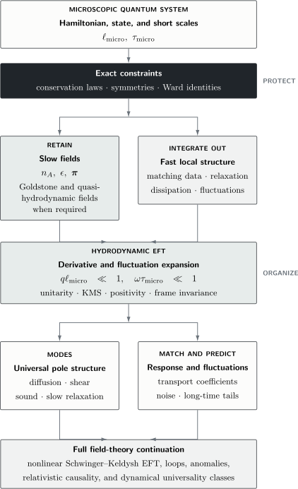

Hydrodynamic EFT retains densities and other parametrically slow fields while integrating out rapidly relaxing structure. Conservation, symmetry, unitarity, KMS, and positivity constrain the derivative expansion; microscopic theory enters through thermodynamics, transport, noise, and matching coefficients.

The diagram separates two kinds of information:

1. Protected structure: conservation laws, symmetries, and Ward identities survive coarse graining.
2. Matched data: equations of state, transport coefficients, relaxation scales, and noise amplitudes depend on microscopic dynamics and the state.

Universality concerns the allowed long-distance structure. It does not imply universal numerical viscosity, conductivity, or diffusion.

Exact Equations and Constitutive Input

For several conserved scalar densities,

$$\partial_t n_A + \partial_i j_A^i = 0.$$

This equation can hold as an operator identity. Hydrodynamics closes it by expressing $j_A^i$ in terms of the retained fields. Near a homogeneous state with no background flow,

$$j_A^i = -L_{AB} \partial_i\lambda_B +\cdots,$$

where $\lambda_B$ are thermodynamic forces, often combinations such as $\mu_B/T$. The ellipsis contains higher gradients, nonlinearities, reversible terms, background-field terms, and noise.

The constitutive relation is not exact because the current is itself a microscopic operator with fast components. It becomes useful after those components have relaxed and their residual effect can be represented by local coefficients.

Conservation with sources and sinks

Background gauge fields or explicit symmetry breaking modify the balance equation. Schematically,

$$\partial_t n_A + \partial_i j_A^i = s_A - \Gamma_{AB}\delta n_B.$$

The source $s_A$ describes injection or extraction. A small relaxation matrix $\Gamma_{AB}$ describes weakly broken conservation. Neither term should be inserted without identifying the microscopic process and its scaling.

Derivative and Amplitude Expansions

Hydrodynamics is commonly organized in derivatives:

$$j_A^i = j_{A,(0)}^i + j_{A,(1)}^i + j_{A,(2)}^i +\cdots.$$

The ideal term $j_{(0)}$ contains no gradients. First-order terms include diffusion, viscosity, and heat conduction. Higher orders encode finite relaxation times, dispersive corrections, and additional tensor structures.

Linearized hydrodynamics also expands in small amplitudes:

$$n_A = n_{A,0} + \delta n_A, \qquad |\delta n_A| \ll |n_{A,0}|.$$

These are independent approximations. A slowly varying flow can be nonlinear in amplitude; a small-amplitude perturbation can vary too rapidly for hydrodynamics. Turbulent or shock-like regimes require nonlinear equations and may invalidate a simple derivative truncation.

Mode-dependent power counting

For sound,

$$\omega \sim q,$$

while for diffusion,

$$\omega \sim q^2.$$

Terms of the same apparent derivative order can therefore contribute differently in different channels. A consistent calculation declares its scaling before deciding which temporal and spatial derivatives to retain.

Diffusion as the Minimal Example

For one conserved scalar density in an isotropic state,

$$\mathbf j = -D\nabla n$$

gives

$$\partial_t n = D\nabla^2 n.$$

A plane wave then has

$$\omega_{\mathrm{diff}} = -iDq^2.$$

The vanishing decay rate at $q=0$ reflects exact conservation. The detailed density response,

$$\chi_{nn}^R(\mathbf q,\omega) = \chi \frac{Dq^2} {Dq^2-i\omega},$$

and its noncommuting static and uniform limits are derived on Transport Coefficients Preview.

Diffusion is not synonymous with incoherence. It is a statement about the long-distance pole. Microscopically, the same $D$ can arise from quasiparticle scattering, chaotic operator dynamics, environmental collisions, or strongly interacting relaxation without sharp carriers.

Momentum, Shear, and Sound

When momentum is conserved, its current is the stress tensor:

$$\partial_t\pi_i + \partial_j\Pi_{ij} = 0.$$

Transverse momentum does not couple to pressure at linear order. In a simple isotropic nonrelativistic fluid,

$$\omega_{\mathrm{shear}} = -i\nu q^2 +\cdots, \qquad \nu = \frac{\eta}{\rho_m}.$$

Here $\eta$ is shear viscosity and $\rho_m$ is mass density.

Longitudinal density and momentum couple. The ideal linear equations can be written

$$\begin{aligned} \partial_t\delta\rho &= -\rho_0 \nabla\boldsymbol\cdot\mathbf v, \\ \rho_0\partial_t\mathbf v &= -\nabla\delta p, \\ \delta p &= c_s^2\delta\rho. \end{aligned}$$

They produce sound. Dissipative gradients shift the poles to

$$\omega_\pm(q) = \pm c_s q - i\Gamma_s q^2 + O(q^3).$$

The coefficient $\Gamma_s$ depends on viscosity, thermal transport, thermodynamic derivatives, dimension, and field content. Its detailed form is not universal and remains with the transport treatment.

If continuous momentum is relaxed by a lattice, substrate, disorder, or bath, ordinary fluid sound and shear need not remain hydrodynamic. Solids can still support phonons because broken translations supply displacement fields. The mechanism selecting the slow field matters more than the name “sound.”

Coupled Diffusion

Suppose several scalar charges are conserved. Linearized constitutive relations lead to

$$\partial_t\delta n_A = D_{AB} \nabla^2\delta n_B.$$

In thermodynamic-force variables,

$$D = L\chi^{-1},$$

where $L$ is a kinetic matrix and $\chi$ the static susceptibility matrix. The eigenvalues of $D$ determine the diffusive eigenmodes. The original particle, spin, or heat densities need not diffuse independently.

Stability requires the eigenvalues relevant to physical perturbations to have nonnegative real parts. In time-reversal-invariant equilibrium, Onsager relations constrain $L$ after the parities of the variables are included. Positivity applies naturally to the dissipative symmetric part in the thermodynamic metric, not to every matrix entry separately.

Diagonalizing $L$ alone can be wrong because susceptibilities convert thermodynamic forces into density perturbations. Diagonalizing $\chi$ alone can be wrong because kinetics selects the decay channels.

Matching Transport Coefficients

Hydrodynamics predicts pole forms but does not calculate every coefficient from symmetry. Matching supplies:

$$\begin{gathered} p(T,\mu_A), \qquad \chi_{AB}, \qquad L_{AB}, \\ \qquad \eta, \qquad \zeta, \qquad \ldots \end{gathered}$$

Possible matching routes include:

• equilibrium thermodynamics for the equation of state and susceptibilities;
• Kubo or Green–Kubo correlation formulas;
• kinetic theory in a controlled quasiparticle regime;
• exact or numerical real-time evolution;
• experiment;
• matching from a more microscopic effective theory.

The matching scale must lie inside an overlap window: below microscopic excitations that have been integrated out, but above the frequencies and wave numbers where the final hydrodynamic prediction is used.

Order of limits

Transport coefficients often involve

$$\begin{aligned} L&\to\infty, & q&\to0, \\ \omega&\to0, & \eta_{\mathrm{reg}}&\to0. \end{aligned}$$

These limits need not commute. A finite isolated system has a discrete spectrum and recurrences; a hydrodynamic pole requires a bulk and long-time regime. A smooth curve produced by arbitrary numerical broadening is not by itself a transport coefficient.

Kubo Formula owns the exact source-response derivation and contact terms. Transport Coefficients Preview owns the coefficient dictionary and finite-size audit.

Hydrodynamics as an Effective Field Theory

Hydrodynamics has the usual EFT ingredients:

• a specified set of low-energy fields;
• symmetries and exact constraints;
• a derivative and fluctuation expansion;
• coefficients matched from shorter scales;
• a cutoff beyond which the description is not trusted;
• field redefinitions that change conventions but not observables.

Its unusual feature is dissipation. A single ordinary real-time action does not naturally encode both causal response and fluctuations while preserving normalization. The in-in construction supplies the needed doubled fields.

Introduce background sources on two branches:

$$\begin{aligned} Z[A_+,A_-;g_+,g_-] &= \operatorname{Tr} \left[ U_+ \rho_0 U_-^{\dagger} \right], \\ U_\pm &\equiv U_{A_\pm,g_\pm}. \end{aligned}$$

The gauge sources $A_\pm$ generate conserved currents. Metric or geometric sources $g_\pm$ generate stress tensors. Equal sources give

$$Z[A,A;g,g] = 1.$$

Gauge invariance yields current Ward identities; diffeomorphism or translation structure yields energy-momentum identities. The effective action must realize these constraints after fast fields are integrated out.

A Diffusive Schwinger–Keldysh Action

In the classical thermal regime, a schematic quadratic action for one density is

$$\begin{aligned} S_{\mathrm{diff}} &= \int dt\,d^d\mathbf x \left[ n_a \left( \partial_t n_r - D\nabla^2n_r \right) \right. \\ &\qquad\left. + iT\chi D \partial_i n_a \partial_i n_a \right]. \end{aligned}$$

The $r$ field is the physical density fluctuation. The $a$ field is a response or difference field. Source terms, initial-state terms, and nonlinear completion are omitted here, so this is a structural preview rather than a standalone microscopic action.

The action displays the characteristic constraints:

$$S_{\mathrm{diff}}[n_r,0] = 0,$$

and

$$\operatorname{Im} S_{\mathrm{diff}} = T\chi D \int dt\,d^d\mathbf x\, (\nabla n_a)^2 \geq 0.$$

The first relation expresses equal-branch normalization. The second damps large difference configurations when $T\chi D\geq0$.

Varying the real part with respect to $n_a$ gives the diffusion equation. The imaginary term is equivalent to a noisy current:

$$\partial_t n_r - D\nabla^2n_r = -\partial_i\xi_i,$$

with

$$\begin{aligned} \langle\xi_i(x)\rangle &= 0, \\ \langle\xi_i(x)\xi_j(x')\rangle &= 2T\chi D\, \delta_{ij} \delta^{(d+1)}(x-x'). \end{aligned}$$

The noise strength is not optional decoration. In equilibrium it is tied to dissipation by fluctuation–dissipation. Removing it while retaining $D$ produces the mean diffusion equation but not the correct equilibrium fluctuations or loop corrections.

Different field normalizations move factors of $\chi$, $T$, and two between the action and sources. The invariant content is the retarded diffusion operator together with a positive noise kernel fixed by the declared equilibrium convention.

Unitarity, KMS, and the Second Law

A hydrodynamic in-in effective action for fields $\Psi_r,\Psi_a$ inherits

$$S_{\mathrm{eff}}[\Psi_r,0] = 0,$$

and a reality relation of the form

$$S_{\mathrm{eff}}[\Psi_r,\Psi_a]^* = -S_{\mathrm{eff}}[\Psi_r,-\Psi_a].$$

The imaginary part must have the sign needed for convergence and positivity. In thermal equilibrium, a dynamical implementation of KMS further relates response and noise. These conditions constrain which dissipative terms can appear and connect them to entropy production and Onsager reciprocity.

At the constitutive level, entropy balance has the schematic form

$$\partial_t s + \partial_i j_s^i = X_M L_{MN} X_N \geq 0,$$

where $X_M$ are thermodynamic forces. Positivity constrains the dissipative symmetric part of $L$. Nondissipative Hall-like or antisymmetric transport can contribute to currents without producing entropy.

The second law is not an independent microscopic proof that every phenomenological coefficient is positive. Its implementation depends on field definitions, equations of motion, anomalies, and allowed improvement terms. Full EFT formulations make these qualifications systematic.

Fluctuating and Nonlinear Hydrodynamics

Hydrodynamic fields fluctuate because a coarse cell contains finitely many microscopic degrees of freedom and exchanges conserved quantities with neighboring cells. Nonlinear constitutive terms couple the slow modes to one another. Schematically,

$$\partial_t\Psi = \mathcal L\Psi + \mathcal N[\Psi,\Psi] + \xi.$$

Loops of hydrodynamic modes can generate:

• algebraic long-time tails;
• nonanalytic dependence on $\omega$ and $q$;
• scale-dependent effective transport coefficients;
• enhanced fluctuations in low spatial dimension;
• corrections that no finite polynomial derivative expansion reproduces term by term.

For a common diffusive mode-coupling channel, a correlation can decay as

$$C(t) \sim t^{-d/2},$$

although the exponent and amplitude depend on the observable and coupled fields. A power-law tail is therefore a prediction of the nonlinear low-energy theory, not automatically evidence for a microscopic quasiparticle.

Hydrodynamic fluctuations are part of the EFT’s dynamics. Treating constitutive equations as noiseless deterministic laws is sufficient for mean linear response in some regimes, but not for fluctuation spectra, higher correlations, or loop-level precision.

Hydrodynamic Frames and Field Redefinitions

Away from strict equilibrium, temperature, chemical potential, and velocity are definitions of effective fields. At derivative order they can be redefined:

$$\begin{aligned} T &\to T+\delta T_{(1)}, \\ \mu_A &\to \mu_A+\delta\mu_{A,(1)}, \\ u^i &\to u^i+\delta u_{(1)}^i. \end{aligned}$$

Such transformations move terms among the constitutive relations. Choosing a Landau, Eckart, mass, entropy, or another frame is a convention for the fields, not a change in the underlying physical state.

Observable currents, response functions, pole locations, and entropy production must be frame invariant to the working order. Comparing two papers coefficient by coefficient before translating frames can create false disagreements.

The EFT analogy is direct: operators proportional to lower-order equations of motion can often be shifted by field redefinitions. A nonredundant basis is defined only after those equivalences are handled.

Approximate Conservation and Quasihydrodynamics

If a charge relaxes slowly,

$$\partial_t n + \nabla\boldsymbol\cdot\mathbf j = -\Gamma n, \qquad \Gamma\tau_{\mathrm{micro}} \ll 1,$$

then its mode becomes

$$\omega = -i\Gamma - iDq^2 +\cdots.$$

It is not exactly hydrodynamic because the pole does not reach the origin at $q=0$, but it remains parametrically slow. Keeping the field explicitly can be much more local than integrating it out.

Examples include weak momentum relaxation, intervalley imbalance, nearly conserved spin, weakly broken integrability, and slow chemical reactions. The relaxation matrix and constitutive coefficients must be expanded in a consistent hierarchy; taking $\Gamma$ large while retaining the field defeats the quasihydrodynamic premise.

Extra Fields in Ordered and Critical Phases

Broken continuous symmetry

A superfluid or magnet with a broken continuous symmetry carries a Goldstone field in addition to conserved densities. The phase can support propagating modes and nondissipative currents. Goldstone Modes in Many-Body Systems owns the symmetry and counting theory.

Superfluidity in Condensed Matter applies this slow-field and constitutive logic to neutral two-fluid materials; this page retains the generic hydrodynamic effective theory.

Solids and viscoelastic media

Broken translations introduce displacement or strain fields. Depending on defect motion and relaxation, a material can behave elastically at short times and hydrodynamically at long times. Ordinary fluid constitutive relations omit this memory.

Critical dynamics

Near a continuous transition, a long-lived order parameter and conserved densities can couple. Static universality alone does not fix the dynamic universality class. Whether the order parameter is conserved and which densities it couples to determine the appropriate Hohenberg–Halperin-type model.

Integrable systems

An integrable system can have an extensive set of conserved quasiparticle occupations. Generalized hydrodynamics evolves a distribution over species and rapidity rather than a short vector of charge densities. Integrability and Generalized Gibbs Ensembles Preview owns that many-body bridge.

Localized systems

An ideal many-body-localized phase does not support ordinary thermal diffusion. Slow dephasing, rare-region effects, finite-size crossover, or external coupling can mimic unusual hydrodynamics over limited windows. The Many-Body Localization Preview owns the stability and diagnostic cautions.

Causality, Stability, and Higher Orders

The diffusion equation has a Gaussian Green function with nonzero support at every distance for any $t>0$. This does not imply that a microscopic local quantum system transmits information instantaneously. Diffusion is an asymptotic equation valid for

$$q \ll \ell_{\mathrm{micro}}^{-1}, \qquad \omega \ll \tau_{\mathrm{micro}}^{-1}.$$

Its exponentially small far tail lies outside the regime in which the truncated equation resolves a microscopic front.

A simple causal completion introduces current relaxation:

$$\tau_J\partial_t\mathbf j + \mathbf j = -D\nabla n.$$

Together with continuity, this gives a telegrapher-type equation. At frequencies below $\tau_J^{-1}$ it reduces to diffusion; near or above that scale, the current is an additional dynamical field.

Relativistic first-order viscous equations can become acausal or unstable when extrapolated beyond their proper regime. Higher-order or transient formulations can repair some problems, but coefficient constraints and mode stability must be checked. “Second order” is not by itself a proof of causality or correctness.

Boundaries, Finite Size, and Initial Data

Hydrodynamics is a boundary-value and initial-value theory. A bulk equation does not determine:

• no-slip, partial-slip, or stress boundary conditions;
• absorbing, reflecting, or reservoir-coupled charge boundaries;
• thermal contact resistance;
• surface modes and edge currents;
• injection profiles;
• the projection of microscopic initial data onto slow fields.

For a finite closed region,

$$\frac{dQ_A}{dt} = -\int_{\partial V} dS_i\, j_A^i.$$

Global conservation follows only when the boundary flux vanishes. In a box of size $L$, the smallest nonzero wave number is of order $L^{-1}$, so a diffusive relaxation time scales as

$$\tau_L \sim \frac{L^2}{D}.$$

Finite-size recurrences and discrete spectra eventually invalidate an infinite-medium decay law. The useful hydrodynamic window lies after local equilibration and before those finite-size effects dominate.

Quantum and Classical Fluctuation Regimes

At nonzero temperature and sufficiently low frequency,

$$\omega \ll T,$$

the KMS factor reduces to its classical form and a stochastic hydrodynamic action is often adequate. This does not make the microscopic system classical. It means the highly occupied low-frequency modes have an effectively classical fluctuation relation.

At $T=0$, near a quantum critical point, or at frequencies comparable to $T$, quantum fluctuation structure remains important. A classical white-noise action need not apply. Superfluids, topological phases, anomalies, and driven open systems can also require additional quantum or geometric data.

Coarse-grained entropy production is compatible with microscopic unitary evolution. Hydrodynamics discards detailed correlations in fast degrees of freedom and follows only a restricted set of observables. The underlying von Neumann entropy of a closed total state need not increase.

Relation to Renormalization and Matching

Hydrodynamics is a Wilsonian idea in real time: integrate out faster and shorter-distance structure while retaining all operators allowed by the symmetries and in-in constraints. Its cutoff satisfies

$$q \lesssim \Lambda_{\mathrm{hydro}} \ll \ell_{\mathrm{micro}}^{-1}.$$

Changing the cutoff shifts effective coefficients so predictions remain invariant to the working order. Nonlinear hydrodynamic loops can make this running explicit.

Near a critical point, the correlation length becomes an additional large scale and critical fluctuations must remain in the EFT. Critical Phenomena and RG Bridge develops the static scaling logic; dynamic critical field theory additionally tracks relaxation and conservation.

The distinction between matching and evolution is essential:

• microscopic theory or data determine the EFT coefficients at a scale;
• hydrodynamic equations evolve the retained fields below that scale;
• renormalization relates descriptions with different cutoffs;
• uncertainty from omitted operators sets the truncation error.

When Full Field Theory Is Needed

The many-body equations on this page are sufficient for identifying slow fields, leading pole structures, and the logic of matching. A full hydrodynamic QFT treatment becomes necessary for:

• nonlinear fluctuating hydrodynamics beyond tree level;
• systematic Schwinger–Keldysh operator bases;
• dynamical KMS and topological unitarity symmetries;
• relativistic fluids and causal transient theories;
• gauge, gravitational, or anomalous backgrounds;
• superfluids, solids, active matter, and reaction networks as complete EFTs;
• critical dynamics and dynamic renormalization groups;
• multi-point response, counting statistics, and noise interactions;
• controlled renormalization of long-time tails.

The Continue on QFT.org crosswalk tracks the planned hydrodynamics, transport, and nonequilibrium destinations and provides the current live fallback.

Method-Selection Guide

Static equilibrium

Use thermodynamics or Euclidean methods for equations of state and static susceptibilities. Hydrodynamic evolution is unnecessary unless a slow spacetime variation is part of the question.

Weak near-equilibrium response

Use Kubo formulas to match coefficients, then hydrodynamics to organize the joint low-$q$, low-$\omega$ response.

Dilute quasiparticle regime

Use Boltzmann transport when a controlled distribution function and collision integral exist. Its moments can match onto hydrodynamics after nonconserved distortions relax.

Strongly interacting long-distance regime

Hydrodynamics can remain valid without quasiparticles if local relaxation and a closed set of slow fields are established.

Finite coherent system

Direct unitary evolution, exact diagonalization, or tensor networks may be more informative before a scale-separated hydrodynamic window appears.

Open or driven system

Include explicit source, sink, noise, and steady-state structure. Ordinary equilibrium KMS and entropy arguments do not transfer automatically.

Integrable or nearly integrable system

Use generalized or quasihydrodynamic variables rather than forcing an extensive slow sector into one diffusion constant.

Reliability Checklist

1. Identify every exact and approximate conservation law.
2. State the equilibrium or steady reference state and ensemble.
3. List retained slow fields and justify omitted candidates.
4. Declare the amplitude, derivative, and fluctuation power counting.
5. Specify the frame and source conventions.
6. Match susceptibilities and transport coefficients in compatible variables.
7. Check stability, positivity, causality within the cutoff, and conservation.
8. Recover KMS and fluctuation–dissipation in equilibrium.
9. Test sensitivity to boundaries, system size, and initial preparation.
10. Estimate higher-gradient, nonlinear, and nonhydrodynamic corrections.

Common Mistakes

1. Calling every slow decay hydrodynamic. A conservation law or parametrically slow field must be identified.
2. Treating a continuity equation as a closed dynamics. The constitutive relation carries the material response.
3. Assuming all conserved densities diffuse independently. Coupled susceptibilities and kinetic matrices determine the eigenmodes.
4. Using momentum hydrodynamics on a lattice without a relaxation audit. Umklapp, disorder, and substrates can remove momentum as a slow field.
5. Equating hydrodynamics with quasiparticle kinetics. Kinetics is one matching route, not a prerequisite for hydrodynamics.
6. Omitting noise from a fluctuation calculation. Dissipation without its equilibrium noise partner violates fluctuation–dissipation.
7. Comparing frame-dependent coefficients directly. Translate field definitions before diagnosing disagreement.
8. Extrapolating diffusion to microscopic fronts. A parabolic long-distance equation does not resolve ultraviolet propagation.
9. Using static universality to infer dynamic universality. Conservation and reversible couplings also select the dynamic class.
10. Ignoring boundaries and limit order. Bulk coefficients do not by themselves determine a finite-device measurement.
11. Treating a white-noise model as quantum at every frequency. Its classical thermal regime must be stated.
12. Calling a derivative truncation exact because it follows symmetry. Symmetry fixes allowed structures, while matching and truncation control accuracy.

Practical Workflow

1. Choose the observables and spacetime regime.
2. Derive or cite the microscopic balance equations.
3. Identify exact, approximate, Goldstone, elastic, or critical slow fields.
4. Construct the most general constitutive relations allowed at the chosen order.
5. Remove frame-redundant terms and fix conventions.
6. Impose equilibrium KMS, Onsager, positivity, and Ward identities where applicable.
7. Match thermodynamics, transport, relaxation, and noise.
8. Linearize and diagonalize only after the full slow sector is assembled.
9. Compare poles, residues, static limits, and equal-time fluctuations with microscopic or experimental data.
10. Increase derivative, nonlinear, and fluctuation order until the desired accuracy is reached or the EFT window closes.

Exercises

Exercise 1: Select the slow fields

For each system, name the minimal hydrodynamic fields and one possible extra slow field:

1. a neutral translation-invariant normal fluid;
2. a dirty electronic conductor with strong momentum relaxation;
3. a neutral superfluid;
4. a system near a nonconserved Ising order-parameter transition;
5. a weakly nonintegrable one-dimensional gas.

Solution

1. Retain energy, mass or particle density, and momentum density. An additional internal charge is included if exactly conserved.
2. Retain charge and energy densities. Momentum can be integrated out only if its relaxation rate is fast compared with the working frequencies; otherwise it is quasihydrodynamic.
3. Retain energy, particle density, momentum, and the superfluid Goldstone phase.
4. Retain energy and any exact charges, plus the slowly relaxing Ising order parameter. Its nonconservation distinguishes its dynamic class from a conserved scalar.
5. Retain the usual exact densities and enough approximately conserved quasiparticle or charge distributions to describe the long prethermal window. Ordinary few-field hydrodynamics may emerge only after integrability-breaking relaxation.

Exercise 2: Diffusion from conservation

Combine

$$\partial_t n + \nabla\boldsymbol\cdot\mathbf j = 0$$

with $\mathbf j=-D\nabla n$. Find the pole of a plane-wave perturbation and explain why its rate vanishes as $q\to0$.

Solution

Substitution gives

$$\partial_t n = D\nabla^2n.$$

For

$$n \propto e^{i\mathbf q\cdot\mathbf x-i\omega t},$$

one obtains

$$-i\omega = -Dq^2,$$

so

$$\omega = -iDq^2.$$

The rate $Dq^2$ vanishes because a long-wavelength density excess cannot decay locally; the conserved quantity must flow over a distance of order $q^{-1}$.

Exercise 3: Ideal sound

Use the three ideal longitudinal equations

$$\begin{aligned} \partial_t\delta\rho &= -\rho_0\nabla\boldsymbol\cdot\mathbf v, \\ \rho_0\partial_t\mathbf v &= -\nabla\delta p, \\ \delta p &= c_s^2\delta\rho \end{aligned}$$

to derive the sound dispersion.

Solution

Differentiate the continuity equation with respect to time and insert the divergence of the momentum equation:

$$\begin{aligned} \partial_t^2\delta\rho &= -\rho_0 \nabla\boldsymbol\cdot \partial_t\mathbf v \\ &= \nabla^2\delta p \\ &= c_s^2\nabla^2\delta\rho. \end{aligned}$$

A plane wave therefore satisfies

$$\omega^2 = c_s^2q^2,$$

so

$$\omega_\pm = \pm c_sq.$$

Viscosity and thermal conduction add attenuation of order $-iq^2$ but do not change the leading ideal propagation speed.

Exercise 4: Weakly broken conservation

Let

$$\partial_t n + \nabla\boldsymbol\cdot\mathbf j = -\Gamma n, \qquad \mathbf j = -D\nabla n.$$

Find the mode frequency and identify the regimes in which $n$ should remain an explicit field.

Solution

The equation becomes

$$\partial_t n = D\nabla^2n - \Gamma n.$$

For a plane wave,

$$\omega = -i \left( \Gamma+Dq^2 \right).$$

If $\Gamma$ is much smaller than microscopic relaxation rates and comparable to the frequencies of interest, $n$ is quasihydrodynamic and should remain explicit. At frequencies and wave numbers far below $\Gamma$, it can often be integrated out, though doing so changes the local operator expansion for the remaining fields.

Exercise 5: Coupled diffusion

Two densities obey

$$\partial_t \begin{pmatrix} n_1 \\ n_2 \end{pmatrix} = \begin{pmatrix} D_1 & \alpha \\ \beta & D_2 \end{pmatrix} \nabla^2 \begin{pmatrix} n_1 \\ n_2 \end{pmatrix}.$$

Find the two diffusion eigenvalues. What stability condition must they satisfy?

Solution

The matrix eigenvalues are

$$\begin{aligned} D_\pm &= \frac{D_1+D_2}{2} \\ &\quad \pm \frac12 \sqrt{ (D_1-D_2)^2 + 4\alpha\beta }. \end{aligned}$$

The modes have

$$\omega_\pm = -iD_\pm q^2.$$

Stability requires the physical eigenvalues to have nonnegative real parts. For a real symmetric diffusion matrix, this reduces to

$$\begin{gathered} D_1\geq0, \qquad D_2\geq0, \\ \qquad D_1D_2-\alpha^2\geq0. \end{gathered}$$

In general the positivity test should be performed in the susceptibility-weighted thermodynamic variables, because $D=L\chi^{-1}$ need not be symmetric in the original density basis.

Exercise 6: Noise required by equilibrium

For one Fourier mode, suppose

$$\dot n_{\mathbf q} = -Dq^2n_{\mathbf q} + \eta_{\mathbf q},$$

with white noise

$$\langle \eta_{\mathbf q}(t) \eta_{-\mathbf q}(t') \rangle = \mathcal A_q \delta(t-t').$$

Demand the equilibrium variance $\langle|n_{\mathbf q}|^2\rangle=T\chi$. Determine $\mathcal A_q$.

Solution

Let

$$C_q(t) = \langle|n_{\mathbf q}(t)|^2\rangle.$$

For an Ornstein–Uhlenbeck mode,

$$\frac{dC_q}{dt} = -2Dq^2C_q + \mathcal A_q.$$

Stationarity and $C_q=T\chi$ give

$$0 = -2Dq^2T\chi + \mathcal A_q.$$

Therefore

$$\mathcal A_q = 2T\chi Dq^2.$$

The factor $q^2$ shows that density noise enters through the divergence of a fluctuating current, preserving the total charge at $q=0$.

Exercise 7: Frame invariance

At first derivative order, redefine the velocity by $u^i\to u^i+\delta u^i_{(1)}$. Explain why individual constitutive coefficients can change while the pole locations of physical correlation functions cannot.

Solution

The redefinition changes how the exact current and stress are decomposed into “ideal” and “derivative” pieces. Terms proportional to $\delta u^i_{(1)}$ move between those pieces, so coefficients attached to a particular decomposition can change.

The full physical currents do not change. Correlation functions are obtained by differentiating with respect to external sources, and their poles are properties of the complete linearized equations. An invertible local field redefinition changes the coordinate description of those equations but not their physical eigenfrequencies to the retained order. A disagreement in a frame-dependent coefficient is meaningful only after both descriptions are translated to the same frame.

Exercise 8: Choose the sufficient theory

Choose among equilibrium thermodynamics, Kubo response, kinetic theory, ordinary hydrodynamics, quasihydrodynamics, generalized hydrodynamics, and full Schwinger–Keldysh EFT:

1. static compressibility;
2. dc conductivity from equilibrium current correlations;
3. dilute-gas viscosity with controlled binary collisions;
4. long-wavelength sound after local equilibration;
5. flow with a very slowly relaxing momentum;
6. an integrable gas with inhomogeneous quasiparticle occupations;
7. nonlinear noise vertices and long-time-tail loops.

Solution

1. Use equilibrium thermodynamics.
2. Use Kubo response with the correct limit order and contact terms.
3. Use kinetic theory, then match its moments to hydrodynamic coefficients if desired.
4. Use ordinary hydrodynamics with density, energy, and momentum fields.
5. Use quasihydrodynamics retaining momentum and its small relaxation rate.
6. Use generalized hydrodynamics.
7. Use a full fluctuating or Schwinger–Keldysh hydrodynamic EFT.

The options form a hierarchy, not a ranking. The sufficient theory is the one that retains the relevant slow information with controlled approximations.

Cross-Links

• Density Operators and Current Operators – microscopic densities, currents, and exact continuity equations.
• Transport Coefficients Preview – diffusion, conductivity, viscosity, sound attenuation, Kubo relations, and limit order.
• Collective Modes – response eigenmodes, damping, hybridization, and spectral diagnostics.
• Relaxation and Thermalization – local equilibration and hydrodynamic slow modes in isolated dynamics.
• Fluctuation–Dissipation Theorem – the equilibrium relation between noise and absorptive response.
• Schwinger–Keldysh Bridge – doubled fields, in-in effective actions, influence functionals, and noise kernels.
• Critical Phenomena and RG Bridge – static universality, relevant operators, and continuum scaling.
• Goldstone Modes in Many-Body Systems – broken-symmetry fields and gapless-mode counting.
• Integrability and Generalized Gibbs Ensembles Preview – extensive conserved data and generalized hydrodynamics.
• Many-Body Localization Preview – the failure of ordinary thermal transport in an ideal localized regime.
• Why Many-Body QM Leads to QFT – the broader route from local operators and collective modes to fields.
• Bridge to QFT – a staged route into quantum field theory.
• Continue on QFT.org – audited routes toward the full nonlinear, relativistic, fluctuating, and effective-field-theory continuation.

References

1. L. Onsager, “Reciprocal Relations in Irreversible Processes. I”, Physical Review 37, 405–426 (1931).
2. L. P. Kadanoff and P. C. Martin, “Hydrodynamic Equations and Correlation Functions”, Annals of Physics 24, 419–469 (1963).
3. P. C. Martin, E. D. Siggia, and H. A. Rose, “Statistical Dynamics of Classical Systems”, Physical Review A 8, 423–437 (1973).
4. P. C. Hohenberg and B. I. Halperin, “Theory of Dynamic Critical Phenomena”, Reviews of Modern Physics 49, 435–479 (1977).
5. W. Israel and J. M. Stewart, “Transient Relativistic Thermodynamics and Kinetic Theory”, Annals of Physics 118, 341–372 (1979).
6. D. Forster, Hydrodynamic Fluctuations, Broken Symmetry, and Correlation Functions, CRC Press (1990).
7. L. D. Landau and E. M. Lifshitz, Fluid Mechanics, 2nd ed., Butterworth-Heinemann (1987).
8. S. Dubovsky, L. Hui, A. Nicolis, and D. T. Son, “Effective Field Theory for Hydrodynamics: Thermodynamics, and the Derivative Expansion”, Physical Review D 85, 085029 (2012).
9. P. Kovtun, “Lectures on Hydrodynamic Fluctuations in Relativistic Theories”, Journal of Physics A 45, 473001 (2012).
10. M. Crossley, P. Glorioso, and H. Liu, “Effective Field Theory of Dissipative Fluids”, Journal of High Energy Physics 09, 095 (2017).
11. F. M. Haehl, R. Loganayagam, and M. Rangamani, “Schwinger–Keldysh Formalism I: BRST Symmetries and Superspace”, Journal of High Energy Physics 06, 069 (2017).
12. A. Lucas and K. C. Fong, “Hydrodynamics of Electrons in Graphene”, Journal of Physics: Condensed Matter 30, 053001 (2018).
13. H. Spohn, Large Scale Dynamics of Interacting Particles, Springer (1991).
14. B. Doyon, “Lecture Notes on Generalised Hydrodynamics”, SciPost Physics Lecture Notes 18 (2020).