Statistical Field Theory Preview

A statistical field theory assigns statistical weights to spatial field configurations and computes equilibrium observables by integrating over those configurations. With a regulator and a dimensionless source $j$, its basic form is

Continue on QFT.org identifies when this static functional language should continue into full RG, thermal QFT, or real-time field theory.

$$\begin{aligned} Z_\Lambda[j] &= \int^\Lambda \mathcal D_\mu\phi \\ &\quad\times \exp\left[ -\mathcal S_\Lambda[\phi] \right] \\ &\quad\times \exp\left[ \int_x j_a(x)\phi_a(x) \right]. \end{aligned}$$

Here $\Lambda$ denotes an ultraviolet cutoff, $\mathcal D_\mu\phi$ is a declared measure, and $\mathcal S_\Lambda$ is dimensionless. For an ordinary thermal theory one often writes

$$\mathcal S_\Lambda[\phi] = \beta \mathcal F_\Lambda[\phi], \qquad \beta = \frac{1}{k_{\mathrm B}T},$$

where $\mathcal F_\Lambda$ is a coarse-grained free-energy functional.

The field theory is not merely the stationary configuration of $\mathcal F_\Lambda$. It is the whole regulated distribution:

$$\mathbb P_\Lambda[d\phi] = \frac{1}{Z_\Lambda[0]} \mathcal D_\mu\phi\, e^{-\mathcal S_\Lambda[\phi]}.$$

Saddles, Gaussian fluctuations, perturbative loops, Monte Carlo samples, and renormalization-group transformations are different ways to analyze that distribution.

Canonical Scope

This page is the canonical bridge for:

• defining a statistical field theory as a regulated measure over field configurations;
• deriving an exact coarse-field weight from a microscopic partition sum by a constrained trace or sum;
• distinguishing microscopic, auxiliary, order-parameter, and collective fields;
• separating the measure, cutoff, dimensionless action, and physical free-energy conventions;
• generating moments and connected correlations with sources;
• relating a physical source to susceptibility and fluctuation formulas;
• distinguishing constrained free energies, Wilsonian actions, and one-particle-irreducible effective actions;
• understanding mean field as a saddle and fluctuations as the rest of the field integral;
• using a finite Gaussian field integral as an exact benchmark;
• separating static statistical fields from stochastic or real-time dynamics;
• relating classical statistical fields, finite-temperature Euclidean quantum fields, dimensional reduction, and quantum–classical mappings;
• identifying exact transformations, truncations, numerical errors, and continuum limits.

Focused pages retain neighboring canonical material:

• Landau–Ginzburg Theory Preview owns the local scalar functional, gradient expansion, stationary profiles, Gaussian correlators, interfaces, and Ginzburg criterion.
• Renormalization Group Preview owns flows, fixed points, relevance, universality classes, and fluctuation-corrected critical scaling.
• Path Integrals for Statistical Mechanics owns the derivation of thermal path integrals from quantum traces.
• Hubbard–Stratonovich Transformation Preview owns exact auxiliary-field decoupling, channel and contour choices, and fermion determinants.
• From Euclidean Time to Euclidean QFT owns thermal circles, field-theory Matsubara modes, reflection positivity, and Lorentzian reconstruction.
• Finite-Temperature QFT Bridge owns the translation from Matsubara field theory to thermal propagators, screening, zero-mode matching, and real-time boundary values.
• Quantum Phase Transitions owns quantum-critical scaling and the role of the dynamical exponent.

The task here is to expose the shared statistical architecture without duplicating those specialized derivations.

Start with a Finite Regulator

A formal product over infinitely many points does not define a measure by itself. Begin with $N$ field variables

$$\boldsymbol\phi = (\phi_1,\ldots,\phi_N)$$

on lattice sites, cells, momentum modes, or another finite basis. A simple noncompact scalar measure is

$$d\mu_N(\phi) = \prod_{i=1}^{N} \frac{d\phi_i}{\mu_i},$$

where each $\mu_i$ supplies the units assigned to that integration variable. The regulated partition function is

$$Z_N = \int d\mu_N(\phi)\, e^{-\mathcal S_N(\phi)}.$$

Other fields require other measures:

• an Ising field uses a sum over $\phi_i=\pm1$;
• a compact phase uses a periodic angular measure;
• a unit vector uses the invariant measure on a sphere;
• a complex field integrates two real components per site;
• a gauge field requires link variables, gauge redundancy, and either a quotient or gauge treatment;
• fermionic fields use Berezin integration rather than a probability measure over ordinary numbers.

The notation $\mathcal D\phi$ is shorthand for a specified limit of such finite objects.

The measure is part of the theory

Under a rescaling

$$\phi_i = c\,\varphi_i,$$

the finite measure changes by

$$\prod_i d\phi_i = |c|^N \prod_i d\varphi_i.$$

The Jacobian contributes $N\ln|c|$ to $\ln Z_N$. It may disappear from some normalized correlators, but it matters for absolute free energies, parameter derivatives, anomalies in more structured transformations, and comparisons between regulators.

A continuum theory is a limiting family

Taking a lattice spacing $a\to0$ while holding every bare coefficient fixed does not generally produce a finite continuum theory. One must specify:

1. which physical correlation lengths and observables are held fixed;
2. how bare couplings depend on $a$ or $\Lambda$;
3. which field normalization is used;
4. what boundary conditions and volume limit are taken;
5. which counterterms or matching conditions are required.

The cutoff may instead remain physical because a coarse-grained theory is only intended below a molecular, lattice, healing, or block scale.

From Microscopic States to a Coarse Field

Let microscopic configurations be denoted by $s$, with energy $H[s]$. Choose a block map

$$\phi_X = \mathcal B_X[s]$$

for cells $X$ of linear size $\ell$. The exact constrained weight of the coarse field can be defined by

$$\begin{aligned} e^{-\mathcal S_\ell[\phi]} &= \mathcal C_\ell \sum_s e^{-\beta H[s]} \\ &\quad\times \prod_X \delta_\ell \left( \phi_X-\mathcal B_X[s] \right). \end{aligned}$$

Here $\delta_\ell$ is the delta function or Kronecker constraint appropriate to the chosen field and measure, and $\mathcal C_\ell$ fixes a convention. Integrating over every $\phi_X$ gives

$$\int\mathcal D_\ell\phi\, e^{-\mathcal S_\ell[\phi]} = \mathcal C_\ell \sum_s e^{-\beta H[s]}.$$

Thus the field representation can preserve the microscopic partition function exactly.

For a quantum model, the sum over $s$ is replaced by a trace, a path-integral configuration sum, or a constrained functional integral. The same logic applies: the field weight is the probability distribution or effective weight induced by the microscopic ensemble and the declared coarse map.

Exact does not mean simple

The exact $\mathcal S_\ell[\phi]$ can contain:

• arbitrarily high powers of $\phi$;
• couplings among many cells;
• nonlocal kernels;
• nonanalytic dependence on momenta or frequency;
• boundary and topology dependence;
• complex phases after integrating out fermions or Berry terms;
• several coupled fields even when one order parameter looks dominant.

A short local polynomial is therefore an approximation unless a special model or limit proves otherwise.

Which observables survive the map?

The coarse distribution determines observables that are functions of $\phi$. A microscopic observable $A[s]$ not fixed by the block map requires its conditional expectation:

$$\overline A_\ell[\phi] = \mathbb E \left[ A[s]\mid \mathcal B[s]=\phi \right].$$

Then

$$\langle A\rangle = \frac{1}{Z_\ell} \int\mathcal D_\ell\phi\, \overline A_\ell[\phi]\, e^{-\mathcal S_\ell[\phi]}.$$

Replacing $\overline A_\ell[\phi]$ by a guessed local function is an additional matching approximation.

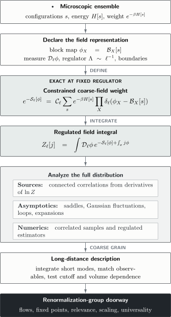
A field representation is fixed by the coarse map, measure, and regulator. The constrained weight can be exact while a local Landau–Ginzburg truncation, a saddle approximation, a loop expansion, or a numerical estimate remains approximate.

A Field Dictionary

The word field does not identify one physical object.

Microscopic field

A lattice spin, occupation, displacement, or second-quantized operator field belongs directly to the microscopic model. Its short-distance algebra and Hilbert space are part of the definition.

Coarse order-parameter field

An order-parameter field is a local average of an operator that transforms in a specified way under a symmetry. It is tied to a source and an observable. Its normalization and block scale must be declared.

Auxiliary field

An auxiliary field is introduced to rewrite an interaction. Before approximation, it is an integration variable whose correlators require matching to physical operators. It may become a useful collective variable, but that is a result rather than a definition.

Collective field

A collective field describes a long-wavelength mode whose correlation function has the relevant pole, soft kernel, or long-range structure. It can be built from microscopic operators, auxiliary fields, constraints, or hydrodynamic densities.

Background source

A source is not integrated over. It is an externally specified field used to define response. Promoting a source to a fluctuating variable changes the theory and requires a measure and action for it.

These categories can be related by matching, but similar symbols do not make them interchangeable.

Order-Parameter Fields and Landau–Ginzburg Theory

Suppose a real scalar order parameter becomes soft near zero wavevector and the long-distance theory is local and analytic. A common dimensionless truncation is

$$\begin{aligned} \mathcal S_{\mathrm{LG}}[\phi;j] &= \int d^d x\, \Bigg[ \frac{c}{2}(\nabla\phi)^2 + \frac{r}{2}\phi^2 \\ &\qquad+ \frac{u}{4!}\phi^4 - j\phi + \cdots \Bigg]. \end{aligned}$$

This expression is not the definition of statistical field theory. It is one important local model within it.

Its form assumes:

• the chosen field captures every relevant soft mode;
• the instability occurs near zero momentum;
• short-distance correlations permit a derivative expansion;
• the omitted powers and gradients are controlled in the regime used;
• the action is stable on the integration domain;
• the cutoff is retained;
• disorder, gauge constraints, long-range forces, and gapless matter do not require a larger nonlocal structure.

Symmetry determines which operators are allowed. It does not determine $r$, $c$, $u$, the cutoff, or the accuracy of the truncation.

The canonical scalar derivations, including the Ornstein–Zernike kernel, correlation length, domain walls, and Ginzburg criterion, remain on Landau–Ginzburg Theory Preview.

Probability Measures and Equilibrium Averages

If $\mathcal S[\phi]$ is real and the weight is nonnegative and normalizable, define

$$\mathbb P[d\phi] = \frac{1}{Z} \mathcal D\phi\, e^{-\mathcal S[\phi]}.$$

For a field functional $A[\phi]$,

$$\langle A\rangle = \frac{1}{Z} \int\mathcal D\phi\, A[\phi]\, e^{-\mathcal S[\phi]}.$$

A sampled field configuration is one equilibrium configuration in the chosen representation. The sequence of configurations generated by a Monte Carlo algorithm is not the system’s physical time evolution.

Positivity is conditional

A real microscopic Hamiltonian does not guarantee that every field representation has a positive weight. Negative or complex factors can arise from:

• fermion determinants or Pfaffians;
• chemical potential and magnetic flux;
• Berry phases and topological terms;
• frustrated basis choices;
• real-time contours;
• auxiliary-field channels with imaginary couplings.

One can still manipulate a signed or complex functional integral, but it is not an ordinary probability measure. Reweighting then involves cancellations and may face a severe sign or phase problem.

Stability and normalizability

A local polynomial potential that tends to $-\infty$ along any real field direction does not define a convergent real-contour measure. Possible resolutions include:

• restoring omitted stabilizing operators;
• restricting a compact field domain;
• identifying that the local expansion was used beyond its range;
• specifying a legitimate complex integration cycle;
• recognizing that the field is a saddle variable rather than a real probability coordinate.

Formal source derivatives cannot repair a divergent measure.

Sources Generate Correlations

Use a dimensionless source convention:

$$\begin{aligned} Z[j] &= \int\mathcal D\phi\, \exp\left[ -\mathcal S[\phi] + \int_x j_a\phi_a \right], \\ W[j] &= \ln Z[j]. \end{aligned}$$

At finite regulator,

$$\frac{\delta W}{ \delta j_a(x) } = \langle\phi_a(x)\rangle_j.$$

A second derivative gives the connected covariance:

$$\begin{aligned} \frac{\delta^2W}{ \delta j_a(x)\delta j_b(y) } &= \langle \phi_a(x)\phi_b(y) \rangle_j \\ &\quad- \langle\phi_a(x)\rangle_j \langle\phi_b(y)\rangle_j. \end{aligned}$$

Higher derivatives generate higher connected cumulants. This is why $W$ is called the connected generating functional.

Physical sources and the factor of beta

Suppose a physical source $h$ enters a thermal free energy as

$$\mathcal F_h[\phi] = \mathcal F_0[\phi] - \int_x h_a(x)\phi_a(x).$$

Then the dimensionless source is

$$j_a(x) = \beta h_a(x).$$

The static susceptibility is therefore

$$\begin{aligned} \chi_{ab}(x,y) &= \frac{\delta \langle\phi_a(x)\rangle }{ \delta h_b(y) } \\ &= \beta \langle \phi_a(x)\phi_b(y) \rangle_{\mathrm c}. \end{aligned}$$

Volume factors, densities, Fourier conventions, and conserved constraints can modify the displayed normalization. The source convention must be stated before a covariance is called a susceptibility.

Exact Gaussian Benchmark

Let $\boldsymbol\phi\in\mathbb R^N$ and let $K$ be a real symmetric positive-definite matrix. Take

$$\mathcal S_0(\phi) = \frac12 \boldsymbol\phi^{\mathsf T} K \boldsymbol\phi.$$

With the measure $d^N\phi$,

$$Z_0[0] = \frac{(2\pi)^{N/2}}{ \sqrt{\det K} }.$$

For a source $\boldsymbol j$,

$$\begin{aligned} Z_0[j] &= Z_0[0] \exp\left( \frac12 \boldsymbol j^{\mathsf T} K^{-1} \boldsymbol j \right), \\ W_0[j] &= W_0[0] + \frac12 \boldsymbol j^{\mathsf T} K^{-1} \boldsymbol j. \end{aligned}$$

It follows that

$$\langle\boldsymbol\phi\rangle_j = K^{-1}\boldsymbol j,$$

and

$$\langle\phi_i\phi_j\rangle_{\mathrm c} = (K^{-1})_{ij}.$$

The covariance is the inverse quadratic kernel. This finite-dimensional identity is the regulated origin of a free field propagator.

Translation-invariant continuum notation

For a scalar field with

$$K(\mathbf q) = r+c\mathbf q^2,$$

the Gaussian covariance is

$$\begin{aligned} \langle \phi_{\mathbf q} \phi_{\mathbf q'} \rangle_{\mathrm c} &= (2\pi)^d \delta^{(d)} (\mathbf q+\mathbf q') \\ &\quad\times \frac{1}{ r+c\mathbf q^2 }. \end{aligned}$$

The pole scale is

$$\xi = \sqrt{\frac{c}{r}}, \qquad r>0.$$

These equations are an exact Gaussian benchmark, not a proof that an interacting critical point is Gaussian.

Mean Field, Saddles, and Fluctuations

Let $\phi_\star$ satisfy

$$\left. \frac{\delta\mathcal S}{ \delta\phi } \right|_{\phi_\star} = 0.$$

Write

$$\phi = \phi_\star+\eta.$$

The action expands as

$$\begin{aligned} \mathcal S[\phi] &= \mathcal S[\phi_\star] \\ &\quad+ \frac12 \eta\mathcal H_\star\eta + \mathcal S_{\mathrm{int}}[\eta], \end{aligned}$$

where $\mathcal H_\star$ is the Hessian. Keeping only $\mathcal S[\phi_\star]$ is the saddle or mean-field approximation. Performing the Gaussian $\eta$ integral gives the first fluctuation determinant.

For one isolated stable saddle with no zero modes,

$$\begin{aligned} -\ln Z &\simeq \mathcal S[\phi_\star] \\ &\quad+ \frac12 \operatorname{Tr} \ln\left( \frac{\mathcal H_\star}{2\pi} \right) + \cdots. \end{aligned}$$

The measure convention determines the constant inside the logarithm. Symmetry zero modes, gauge directions, negative modes, boundaries, and multiple saddles require separate treatment.

Finite volume restores symmetry

Suppose a finite system has a symmetric double-well weight. The two dominant saddles at $\pm\phi_0$ contribute equally at zero source, so

$$\langle\phi\rangle = 0$$

even when a one-saddle approximation reports $\phi_0$. Spontaneous symmetry breaking requires an order of limits, source prescription, or invariant long-range diagnostic. A saddle is a candidate phase sector, not the exact finite-volume average.

Criticality defeats naive Gaussian control

As a Hessian eigenvalue approaches zero, fluctuations in that direction grow. The Gaussian determinant becomes infrared sensitive, interaction vertices can become important, and a loop expansion about the mean-field saddle may lose control. This is the point where the Ginzburg criterion and renormalization-group analysis become essential.

Three Objects Called an Effective Action

The phrase effective action is overloaded. A reliable derivation names the object being used.

Constrained coarse-field functional

The functional $\mathcal S_\ell[\phi]$ defined by a delta constraint is the negative logarithm of the probability density for a declared coarse field. It depends on the block map and scale $\ell$.

Wilsonian action

Split a regulated field into retained and removed modes:

$$\phi = \phi_<+\phi_>.$$

Define

$$\begin{aligned} e^{-\mathcal S_{\Lambda'}[\phi_<]} &= \int_{\Lambda'<|q|<\Lambda} \mathcal D\phi_> \\ &\quad\times e^{-\mathcal S_\Lambda[ \phi_<+\phi_> ]}. \end{aligned}$$

The Wilsonian action is still used inside an integral over the retained field. Integrating out modes generally changes every allowed coupling and generates new operators.

One-particle-irreducible effective action

Define the mean field

$$m_a(x) = \frac{\delta W[j]}{ \delta j_a(x) }.$$

The Legendre transform is

$$\Gamma[m] = \sup_j \left[ \int_x j_a m_a - W[j] \right].$$

Where differentiable,

$$\frac{\delta\Gamma}{ \delta m_a(x) } = j_a(x).$$

Its second derivative is the inverse connected two-point function on the appropriate subspace. At finite volume the exact Legendre effective potential is convex, even when a bare Landau polynomial or a one-saddle approximation has a double-well shape.

The constrained functional, Wilsonian action, and $\Gamma$ can be related. They are not identical at an arbitrary scale or approximation.

Coarse Graining as the Next Step

One exact integration over short modes produces $\mathcal S_{\Lambda'}$. To compare it with the original theory, one then rescales coordinates, fields, and couplings. Repetition produces a trajectory through a space of actions.

This page stops at that doorway. The classification of:

• fixed points;
• relevant, irrelevant, and marginal directions;
• scaling dimensions;
• universality;
• corrections to scaling;
• upper critical dimensions;
• nonperturbative flows

belongs on Renormalization Group Preview. Critical Phenomena and RG Bridge then translates fixed points, eigenoperators, and relevant deformations into continuum-QFT language.

The important lesson here is narrower: coarse graining is an integration over fluctuations, not a verbal instruction to smooth a plot.

Static Theory Is Not Dynamics

The equilibrium measure

$$\mathbb P[d\phi] \propto \mathcal D\phi\, e^{-\mathcal S[\phi]}$$

does not determine how $\phi$ evolves in physical time. Two systems can share the same equilibrium action and have different dynamics because:

• one order parameter is conserved and another is not;
• momentum or energy is an additional slow variable;
• reversible Poisson-bracket terms differ;
• gauge fields or hydrodynamic modes couple differently;
• the environment changes noise and dissipation.

A stochastic equation such as

$$\partial_t\phi = -\Gamma \frac{\delta\mathcal F}{ \delta\phi } + \zeta$$

adds a kinetic law, mobility, and noise. Equilibrium requires a compatible fluctuation–dissipation relation. None of these follows from the static functional alone.

Likewise, a Monte Carlo update time is algorithmic. It generally has no direct conversion to the physical $t$ in a dynamical equation.

Classical Statistical Fields and Euclidean Quantum Fields

The two structures look similar:

$$Z_{\mathrm{cl}} = \int\mathcal D\phi\, e^{-\beta\mathcal F[\phi]},$$

and

$$Z_{\mathrm q} = \int_{\mathrm{thermal\ bc}} \mathcal D\varphi\, e^{-S_{\mathrm E}[\varphi]/\hbar}.$$

The first integrates fields over $d$ spatial dimensions. The second describes a $d$-dimensional quantum system using fields on space and a compact imaginary time

$$0 \le \tau < \beta\hbar.$$

The mathematical analogy does not erase the differences:

• imaginary time encodes operator ordering and the thermal trace;
• bosons and fermions obey different temporal boundary conditions;
• a Euclidean measure must satisfy additional conditions to reconstruct a Lorentzian quantum theory;
• complex phases and fermion signs can prevent a positive probability interpretation;
• analytic continuation acts on correlation functions, not individual field configurations.

Dimensional Reduction

Expand a periodic bosonic Euclidean field as

$$\varphi(\mathbf x,\tau) = \sum_{n\in\mathbb Z} \varphi_n(\mathbf x) e^{-i\nu_n\tau},$$

with

$$\nu_n = \frac{2\pi n}{ \beta\hbar }.$$

For static observables at spatial momenta much smaller than the nonzero Matsubara scale, modes with $n\ne0$ can sometimes be integrated out. The remaining theory has the form

$$Z_{\mathrm{static}} = \int\mathcal D\varphi_0\, e^{-\mathcal S_d[\varphi_0]}.$$

It is a $d$-dimensional statistical field theory whose coefficients already contain quantum and thermal effects from the removed modes.

Dimensional reduction requires:

• a bosonic zero mode;
• separation between the zero and nonzero mode scales;
• control of additional soft fields;
• matching of all induced operators;
• compatible gauge and boundary constraints;
• an infrared theory that remains well defined.

Thermal fermions have no zero Matsubara mode, but integrating them out can change the static coefficients or generate nonlocal interactions. A fermionic microscopic system can therefore have a bosonic static critical theory without fermions being irrelevant to matching.

Quantum–Classical Correspondence

Product formulas can map a $d$-dimensional quantum partition function to an anisotropic classical model with one additional discrete direction. In a transfer-matrix formulation,

$$Z_{\mathrm{cl}} = \operatorname{Tr} \mathsf T^{N_\tau}.$$

When the transfer matrix is positive and its logarithm is well defined, one may write

$$\mathsf T = e^{-a_\tau H_{\mathrm q}/\hbar},$$

so that the classical layer direction acts like imaginary time.

This correspondence is not the assertion that every $(d+1)$-dimensional classical model is literally the same physical system as a $d$-dimensional quantum model. The mapping fixes:

• anisotropic couplings;
• the Hilbert space and transfer matrix;
• temporal boundary conditions;
• observables that correspond under the map;
• limits needed to remove the time lattice.

At a zero-temperature quantum critical point, imaginary time becomes unbounded and can scale as

$$\tau \longmapsto b^z\tau.$$

The phrase “effective dimension $d+z$” is useful for some power counting and hyperscaling statements. It is not a universal replacement of anisotropic or nonlocal quantum dynamics by an isotropic classical model.

Finite Volume and Boundaries

A field integral must specify:

• spatial volume and shape;
• periodic, open, fixed, free, twisted, or mixed boundaries;
• topological sectors;
• treatment of zero modes;
• source behavior at the boundary;
• order of thermodynamic, continuum, and zero-source limits.

At finite volume, a stable regulated partition function is usually analytic in ordinary parameters. Sharp phase transitions arise through an infinite degree-of-freedom limit, not from drawing a nonconvex saddle potential at one finite size.

Boundary conditions can alter:

• the allowed momenta;
• surface operators and universality classes;
• degeneracies and tunneling between saddles;
• finite-size scaling functions;
• topological sectors;
• whether a nominal zero mode exists.

Numerical Statistical Field Theory

A lattice field calculation typically samples

$$P[\phi] \propto e^{-\mathcal S_{\mathrm{lat}}[\phi]}.$$

Useful algorithms include local Metropolis updates, heat-bath updates, cluster methods, worm or loop methods, hybrid molecular-dynamics methods, and specialized constrained or gauge updates. The action does not select the algorithm automatically.

A reproducible computation reports:

1. lattice action, measure, and boundary conditions;
2. lattice spacing, volume, and aspect ratio;
3. update algorithm and proposal parameters;
4. thermalization and autocorrelation diagnostics;
5. estimator definitions and covariance treatment;
6. finite-size and cutoff extrapolations;
7. sign, phase, or reweighting diagnostics;
8. tests against exact Gaussian, weak-coupling, symmetry, or small-volume limits.

Critical slowing down can make a positive measure hard to sample near a continuous transition. Absence of a sign problem does not imply independent samples or rapid equilibration.

Exact and Approximate Steps

The following statements have different status.

• Exact at fixed regulator: insert a normalized delta constraint, change variables with its Jacobian, integrate a Gaussian field, integrate a finite set of modes, or differentiate a convergent generating functional.
• Representation dependent: choose a coarse variable, block map, field normalization, regulator, boundary condition, or auxiliary channel.
• Controlled only with an argument: truncate to local operators, take a derivative expansion, keep a loop order, use a large-component expansion, or remove the cutoff.
• Saddle approximation: replace the whole field distribution by one or several stationary configurations.
• Statistical estimate: approximate a regulated expectation with correlated Monte Carlo samples.
• Infrared inference: use finite systems and nonzero masses to infer a critical point, continuum limit, or universality class.

An exact field representation can be followed by an uncontrolled truncation. A phenomenological field theory can also be highly predictive when its symmetry, scale window, and fitted coefficients are stated honestly.

Reliable Workflow

1. Define the question

State the observables, distances, temperatures, and precision required.

2. Choose the field

Give its microscopic operator or block-map definition, transformation law, units, and source.

3. Declare the regulator

Specify the lattice, basis, cutoff, volume, boundaries, and measure.

4. Derive or match the weight

Distinguish an exact constrained functional, an auxiliary-field action, and a phenomenological Landau–Ginzburg model.

5. Enumerate allowed operators

Use symmetry and locality, then state why omitted fields, powers, gradients, or nonlocal kernels are suppressed.

6. Choose an evaluation method

Identify the saddle parameter, loop counting, large-$N$ limit, numerical algorithm, or exact structure.

7. Match observables

Relate field correlators and vertices to physical densities, order parameters, susceptibilities, and scattering conventions.

8. Test limits

Check Gaussian, decoupled, atomic, high-temperature, low-density, symmetry, and finite-size benchmarks where available.

9. Separate limits

Do not silently interchange zero source, infinite volume, zero lattice spacing, low frequency, and long distance.

10. Quantify omitted physics

Vary cutoff, field normalization, truncation, channel, volume, and fitting window when those variations diagnose uncertainty.

Common Mistakes

• Writing $\mathcal D\phi$ without a regulator or measure convention.
• Mixing an energy functional $\mathcal F$ with a dimensionless action $\mathcal S=\beta\mathcal F$.
• Calling the minimum of a functional the statistical field theory while omitting the fluctuation integral.
• Treating a coarse field as the microscopic operator at every point.
• Equating an auxiliary variable with an order parameter without source matching.
• Assuming symmetry fixes nonuniversal coefficients.
• Treating a local polynomial as exact after integrating out gapless matter.
• Dropping Jacobians because they cancel in one normalized observable.
• Using a signed or complex Euclidean weight as an ordinary probability.
• Confusing the Monte Carlo update history with physical dynamics.
• Inferring kinetics or a dynamical exponent from a static free energy.
• Calling every coarse functional, Wilsonian action, and Legendre effective action the same object.
• Reading a nonconvex mean-field potential as the exact finite-volume effective potential.
• Assuming every finite-temperature quantum theory dimensionally reduces.
• Forgetting that thermal fermions affect matching despite lacking a zero Matsubara mode.
• Treating $d+z$ as a literal isotropic dimension in every quantum critical problem.
• Removing the cutoff without specifying a matching or renormalization trajectory.

Connections

• Partition Functions supplies the trace and thermodynamic normalization from which field representations begin.
• Path Integrals for Statistical Mechanics derives configuration integrals from quantum thermal traces.
• Landau–Ginzburg Theory Preview develops the central local order-parameter model in detail.
• Order Parameters owns operator, source, symmetry, and thermodynamic-limit definitions.
• Connected Correlation Functions owns cumulants, clustering, and correlation-length estimators.
• Susceptibilities owns static and dynamical response conventions.
• Hubbard–Stratonovich Transformation Preview gives the exact auxiliary-field route into a statistical field integral.
• From Euclidean Time to Euclidean QFT develops the additional conditions required of Euclidean quantum fields.
• Renormalization Group Preview continues from one coarse-graining step to fixed points and universality.

References

1. L. P. Kadanoff, “Scaling Laws for Ising Models near $T_c$”, Physics Physique Fizika 2, 263–272 (1966) – block variables and scale-dependent critical description.
2. K. G. Wilson, “Renormalization Group and Critical Phenomena. I. Renormalization Group and the Kadanoff Scaling Picture”, Physical Review B 4, 3174–3183 (1971) – coarse graining as a transformation of effective interactions.
3. K. G. Wilson, “Renormalization Group and Critical Phenomena. II. Phase-Space Cell Analysis of Critical Behavior”, Physical Review B 4, 3184–3205 (1971) – phase-space-cell formulation and critical behavior.
4. F. J. Wegner and A. Houghton, “Renormalization Group Equation for Critical Phenomena”, Physical Review A 8, 401–412 (1973) – functional integration of momentum shells.
5. K. G. Wilson and J. Kogut, “The Renormalization Group and the $\epsilon$ Expansion”, Physics Reports 12, 75–200 (1974) – statistical fields, coarse graining, and the field-theory bridge.
6. M. E. Fisher, “The Renormalization Group in the Theory of Critical Behavior”, Reviews of Modern Physics 46, 597–616 (1974) – critical correlations, scaling, and universality.
7. M. Suzuki, “Relationship between $d$-Dimensional Quantal Spin Systems and $(d+1)$-Dimensional Ising Systems”, Progress of Theoretical Physics 56, 1454–1469 (1976) – product-formula quantum–classical correspondence.
8. P. C. Hohenberg and B. I. Halperin, “Theory of Dynamic Critical Phenomena”, Reviews of Modern Physics 49, 435–479 (1977) – why static universality does not determine dynamics.
9. J. B. Kogut, “An Introduction to Lattice Gauge Theory and Spin Systems”, Reviews of Modern Physics 51, 659–713 (1979) – transfer matrices and classical–quantum lattice correspondences.
10. P. M. Chaikin and T. C. Lubensky, Principles of Condensed Matter Physics, Cambridge University Press (1995) – order parameters, fields, defects, and fluctuations.
11. J. Cardy, Scaling and Renormalization in Statistical Physics, Cambridge University Press (1996) – field measures, scaling, and renormalization.
12. M. Kardar, Statistical Physics of Fields, Cambridge University Press (2007) – functional integrals, Gaussian fields, interacting theories, and stochastic dynamics.
13. N. Goldenfeld, Lectures on Phase Transitions and the Renormalization Group, CRC Press reissue – coarse graining and critical field theory.

Exercises

1. Preserve the Partition Function

Starting from the constrained definition of $e^{-\mathcal S_\ell[\phi]}$, integrate over $\phi$ and show that the microscopic partition function is preserved when every constraint is normalized.

Solution

Begin with

$$\begin{aligned} \int\mathcal D_\ell\phi\, e^{-\mathcal S_\ell[\phi]} &= \mathcal C_\ell \sum_s e^{-\beta H[s]} \\ &\quad\times \int\mathcal D_\ell\phi \\ &\quad\times \prod_X \delta_\ell \left( \phi_X-\mathcal B_X[s] \right). \end{aligned}$$

Normalization of each constraint gives

$$\int d\mu_X(\phi_X)\, \delta_\ell \left( \phi_X-\mathcal B_X[s] \right) = 1.$$

Therefore

$$\int\mathcal D_\ell\phi\, e^{-\mathcal S_\ell[\phi]} = \mathcal C_\ell \sum_s e^{-\beta H[s]}.$$

Choosing $\mathcal C_\ell=1$ preserves the partition function exactly. Another field-independent convention shifts the absolute free energy and must be retained if that quantity is compared.

2. Gaussian Generating Functional

For the finite positive-definite Gaussian action

$$\mathcal S_0 = \frac12 \boldsymbol\phi^{\mathsf T} K \boldsymbol\phi,$$

derive $Z_0[j]$, the mean field, and the connected covariance.

Solution

Complete the square:

$$\begin{aligned} &-\frac12 \boldsymbol\phi^{\mathsf T} K \boldsymbol\phi + \boldsymbol j^{\mathsf T} \boldsymbol\phi \\ &\quad= -\frac12 (\boldsymbol\phi-K^{-1}\boldsymbol j)^{\mathsf T} K (\boldsymbol\phi-K^{-1}\boldsymbol j) \\ &\qquad+ \frac12 \boldsymbol j^{\mathsf T} K^{-1} \boldsymbol j. \end{aligned}$$

The translated Gaussian has the same normalization, so

$$Z_0[j] = Z_0[0] \exp\left( \frac12 \boldsymbol j^{\mathsf T} K^{-1} \boldsymbol j \right).$$

Thus

$$\frac{\partial W_0}{ \partial j_i } = (K^{-1}\boldsymbol j)_i,$$

and

$$\frac{\partial^2W_0}{ \partial j_i\partial j_j } = (K^{-1})_{ij}.$$

At zero source the mean vanishes and the inverse kernel is the covariance.

3. Physical Source versus Dimensionless Source

A magnetic field $h_i$ enters a coarse free energy as $-\sum_i h_i\phi_i$. Derive the relation between covariance and static susceptibility.

Solution

The thermal weight is

$$\exp\left[ -\beta\mathcal F_0[\phi] + \beta\sum_i h_i\phi_i \right].$$

Hence the dimensionless source is

$$j_i = \beta h_i.$$

Using

$$\frac{\partial\langle\phi_i\rangle}{ \partial j_j } = \langle\phi_i\phi_j\rangle_{\mathrm c},$$

the chain rule gives

$$\chi_{ij} \equiv \frac{\partial\langle\phi_i\rangle}{ \partial h_j } = \beta \langle\phi_i\phi_j\rangle_{\mathrm c}.$$

If $\phi_i$ is a density, a block average, or an extensive total, additional cell-volume conventions must be included consistently.

4. Field Rescaling and the Jacobian

For $N$ noncompact real variables, set $\phi_i=c\varphi_i$. Show how the partition function transforms. Why can one not discard the Jacobian when computing an absolute free energy?

Solution

The measure obeys

$$d^N\phi = |c|^N d^N\varphi.$$

Therefore

$$Z = |c|^N \int d^N\varphi\, e^{-\mathcal S(c\varphi)}.$$

The free energy is

$$F = -k_{\mathrm B}T\ln Z,$$

so the Jacobian contributes

$$\Delta F = -Nk_{\mathrm B}T\ln|c|.$$

It may cancel between numerator and denominator of a normalized expectation that is transformed consistently. It does not cancel from the absolute partition function or from derivatives when $c$ depends on a physical parameter.

5. Two Saddles in Finite Volume

Consider an even one-variable action with two equal minima at $\phi=\pm\phi_0$. Show why the exact zero-source mean vanishes even though a one-saddle approximation does not.

Solution

Because

$$\mathcal S(-\phi) = \mathcal S(\phi),$$

the numerator of the exact mean is odd:

$$\int_{-\infty}^{\infty} d\phi\, \phi e^{-\mathcal S(\phi)} = 0.$$

Hence $\langle\phi\rangle=0$. In a steepest-descent approximation, the two neighborhoods contribute

$$Z \simeq Z_++Z_-,$$

with equal $Z_+=Z_-$. Their contributions to the numerator are opposite and cancel. Keeping only the $+\phi_0$ saddle gives a nonzero result because it has selected one phase sector. Spontaneous order requires a source and thermodynamic-limit prescription or an invariant correlation diagnostic.

6. Classify Three Effective Objects

Classify each construction as constrained, Wilsonian, or one-particle irreducible:

1. insert a delta function fixing block magnetization;
2. integrate momenta between $\Lambda'$ and $\Lambda$;
3. Legendre transform $W[j]$.

Solution

The delta-function construction gives the constrained coarse-field functional: it is the negative logarithm of the induced distribution of the chosen block variable.

Integrating a momentum shell gives the Wilsonian action $\mathcal S_{\Lambda'}$. It remains inside a path integral over lower momenta.

The Legendre transform gives the one-particle-irreducible effective action $\Gamma[m]$. Its derivatives generate inverse connected functions and proper vertices.

The three objects can coincide in special limits or approximations, but they are not synonyms by definition.

7. Bosonic and Fermionic Zero Modes

Derive the bosonic and fermionic Matsubara frequencies and explain why a static fermion mode is absent.

Solution

A periodic bosonic field satisfies

$$\varphi(\tau+\beta\hbar) = \varphi(\tau).$$

For a Fourier mode $e^{-i\nu\tau}$ this requires

$$e^{-i\nu\beta\hbar} = 1,$$

so

$$\nu_n = \frac{2\pi n}{ \beta\hbar }, \qquad n\in\mathbb Z.$$

The $n=0$ mode is static. A thermal fermion is antiperiodic:

$$\psi(\tau+\beta\hbar) = -\psi(\tau).$$

Thus

$$\omega_n = \frac{(2n+1)\pi}{ \beta\hbar },$$

which never vanishes. Fermions can still change the static bosonic action when they are integrated out.

8. Static Measure versus Dynamics

Two systems have the same equilibrium free-energy functional $\mathcal F[\phi]$. In system A, $\phi$ is nonconserved; in system B, it is a conserved density. Explain why their equilibrium correlations can agree while their long-time dynamics differ.

Solution

The same equilibrium measure

$$\mathbb P[d\phi] \propto \mathcal D\phi\, e^{-\beta\mathcal F[\phi]}$$

gives the same static equal-time field correlations.

A nonconserved field can relax locally through a law of the form

$$\partial_t\phi \sim -\Gamma \frac{\delta\mathcal F}{ \delta\phi } + \zeta.$$

A conserved density must obey a continuity equation. Its simplest dissipative law has additional gradients:

$$\partial_t\phi \sim \nabla\cdot \left[ M\nabla \frac{\delta\mathcal F}{ \delta\phi } \right] + \nabla\cdot\boldsymbol\zeta.$$

Conservation therefore changes the small-wavevector relaxation rate and the dynamic universality class without changing the static Gibbs measure.