Finite-Temperature QFT Bridge

Finite-temperature quantum field theory studies a quantum field theory in a thermal state. The local fields and ultraviolet theory remain quantum field theoretic, while the state introduces an inverse temperature $\beta$, a preferred rest frame, thermal occupation factors, and a compact imaginary-time direction.

In natural units,

$$\hbar = c = k_{\mathrm B} = 1,$$

the equilibrium starting point is

$$\begin{aligned} \mathcal Z(\beta,\mu) &= \operatorname{Tr} \exp \left[ -\beta \left( H-\mu Q \right) \right] \\ &= \int_{\mathrm{thermal}} \mathcal D\Phi\, e^{-S_E[\Phi]}. \end{aligned}$$

The subscript on the functional integral carries real content. Bosonic fields are periodic and physical fermion fields are antiperiodic around the Euclidean thermal circle:

$$\begin{aligned} \phi(\tau+\beta,\mathbf x) &= \phi(\tau,\mathbf x), \\ \psi(\tau+\beta,\mathbf x) &= -\psi(\tau,\mathbf x). \end{aligned}$$

The corresponding frequencies are discrete:

$$\omega_n = 2\pi nT, \qquad \widetilde\omega_n = (2n+1)\pi T.$$

These formulas are not an extra postulate attached to zero-temperature QFT. They encode the Kubo–Martin–Schwinger condition and the statistics of fields inside a thermal trace.

Purpose and Canonical Scope

This page owns the translation from the many-body thermal toolkit to the working language of thermal QFT. It explains:

• what changes when a QFT is placed in a thermal state;
• how the thermal circle becomes a field-theory spacetime;
• how Matsubara sums replace loop-energy integrals;
• how thermal propagators separate vacuum and population effects;
• how KMS analyticity relates Euclidean and real-time correlators;
• why screening masses and real-time pole data are distinct;
• when bosonic zero modes lead to a lower-dimensional effective theory;
• where equilibrium imaginary-time methods end and real-time contours begin.

The detailed ingredients retain one canonical home each:

• Finite-Temperature QM Overview owns the common map from Gibbs operators to imaginary time, spectra, and path integrals.
• Imaginary Time owns the operator semigroup, heat-equation form, thermal trace, and projection interpretation.
• Matsubara Formalism Preview owns the compact-time transform, frequency sums, convergence prescriptions, and QM-level workflow.
• Bosonic and Fermionic Matsubara Frequencies owns the explicit-$\hbar$ grids, index arithmetic, parity classification, and finite-cutoff conventions.
• Thermal Green Functions owns graded ordering, equal-time contacts, and detailed free-mode benchmarks.
• Spectral Representation owns thermal Lehmann weights, Cauchy transforms, retarded boundary values, and exact static terms.
• Analytic Continuation owns the finite-data inverse problem, covariance, regularization, and resolution claims.
• From Euclidean Time to Euclidean QFT owns field wavefunctionals, reflection positivity, and the conditions for Lorentzian reconstruction.
• Diagrammatic Methods Preview owns graph combinatorics, line and vertex bookkeeping, self-energies, and diagrammatic double counting.

The purpose here is to expose the field-theory architecture and its limits, not to repeat those derivations.

Convention Ledger

Except where an explicit factor is restored, this page uses natural units. Then

$$\beta = \frac1T, \qquad 0 \leq \tau \lt \beta.$$

We use $d$ for the number of spatial dimensions and

$$D = d+1$$

for Euclidean spacetime dimension before any thermal dimensional reduction. The equilibrium generator is

$$\mathcal K = H-\mu Q,$$

where $Q$ is a conserved charge:

$$[H,Q] = 0.$$

The heat bath selects a timelike four-velocity $u^\mu$. In its rest frame,

$$u^\mu = (1,\mathbf 0).$$

Temperature-dependent formulas should state whether energies are measured relative to $H$ or to $\mathcal K$. A chemical potential can be moved between the density operator, time evolution, and a temporal background field, but the resulting frequency shifts and boundary conditions must be translated consistently.

What Temperature Changes

Finite temperature does not normally mean replacing the QFT Lagrangian by an unrelated thermal Lagrangian. It means evaluating observables in the state

$$\rho_{\beta,\mu} = \frac{ e^{-\beta(H-\mu Q)} }{ \mathcal Z(\beta,\mu) }.$$

This changes correlation functions:

$$\langle \mathcal O_1\cdots\mathcal O_n \rangle_{\beta,\mu} = \operatorname{Tr} \left( \rho_{\beta,\mu} \mathcal O_1\cdots\mathcal O_n \right).$$

It also changes which symmetries the state realizes. Even if the microscopic QFT is Lorentz invariant, a thermal state is not invariant under boosts. In the bath rest frame, spatial rotations may remain unbroken while temporal and spatial tensor structures separate.

For example, a finite-temperature self-energy can depend independently on

$$\omega \qquad\text{and}\qquad \lvert\mathbf k\rvert,$$

rather than only on the Lorentz invariant

$$p^2 = \omega^2-\mathbf k^2.$$

This is why vacuum mass, static screening mass, propagating pole energy, and damping rate need not coincide.

Temperature introduces physical scales:

$$T, \qquad 2\pi T, \qquad \pi T,$$

as well as interaction-generated scales such as a screening mass. A calculation must compare external energies, momenta, masses, and couplings with these scales before choosing an expansion.

From a Trace to a Field Theory on a Thermal Circle

For a bosonic field with Euclidean action $S_E$, the partition function has the schematic form

$$\mathcal Z = \int_{\phi(\beta)=\phi(0)} \mathcal D\phi\, e^{-S_E[\phi]}.$$

For a relativistic scalar,

$$\begin{aligned} S_E[\phi] &= \int_0^\beta d\tau \int d^d x \\ &\quad\times \Biggl[ \frac12 \left( \partial_\tau\phi \right)^2 + \frac12 \left( \boldsymbol\nabla\phi \right)^2 \\ &\qquad\quad + \frac12m^2\phi^2 + \frac{\lambda}{4!}\phi^4 \Biggr]. \end{aligned}$$

The Euclidean spacetime is

$$S^1_\beta \times \mathcal M_d,$$

where the circle circumference is $\beta$. This geometry differs from vacuum Euclidean QFT on noncompact Euclidean time. The zero-temperature limit

$$\beta \longrightarrow \infty$$

decompactifies the circle.

The same construction for physical fermions uses Grassmann fields with antiperiodic temporal boundary conditions:

$$\mathcal Z_{\mathrm F} = \int_{\psi(\beta)=-\psi(0)} \mathcal D\bar\psi\, \mathcal D\psi\, e^{-S_E[\bar\psi,\psi]}.$$

The sign originates in the fermionic trace, not merely in the fact that the integration variables anticommute. This distinction matters in gauge theory: Faddeev–Popov ghosts are Grassmann valued, yet in common thermal covariant gauges they carry periodic thermal frequencies so that gauge identities are maintained. Statistics, field role, and gauge fixing must be considered together.

KMS Is the Equilibrium Principle

Let real-time evolution be

$$\alpha_t(A) = e^{i\mathcal Kt} A e^{-i\mathcal Kt}.$$

For suitable operators, define

$$\begin{aligned} C_{AB}^{>}(t) &= \left\langle \alpha_t(A)B \right\rangle_\beta, \\ C_{AB}^{<}(t) &= \left\langle B\alpha_t(A) \right\rangle_\beta. \end{aligned}$$

The KMS boundary relation is

$$C_{AB}^{>}(t) = C_{AB}^{<}(t+i\beta).$$

With the Fourier convention

$$\widetilde C(\omega) = \int_{-\infty}^{\infty} dt\, e^{i\omega t} C(t),$$

the corresponding detailed-balance relation is

$$\widetilde C_{AB}^{<}(\omega) = e^{-\beta\omega} \widetilde C_{AB}^{>}(\omega).$$

The analytic strip, detailed balance, thermal periodicity, and fluctuation–dissipation relations are consequences of the same equilibrium structure. They are not independent assumptions.

In an infinite-volume QFT, a global trace and density matrix can fail to exist. The KMS condition remains meaningful as a condition on the observable algebra and its time evolution. This is one reason KMS language is more fundamental than the finite-box mnemonic

$$\rho_\beta \propto e^{-\beta H}.$$

KMS Condition Preview owns the finite Gibbs derivation, analytic-strip qualifications, and algebraic bridge.

Matsubara Modes of Fields

A periodic scalar field has the expansion

$$\phi(\tau,\mathbf x) = T \sum_{n\in\mathbb Z} \int_{\mathbf k} e^{i\omega_n\tau+i\mathbf k\cdot\mathbf x} \phi_n(\mathbf k),$$

where

$$\omega_n = 2\pi nT,$$

and

$$\int_{\mathbf k} := \int \frac{d^d k}{(2\pi)^d}.$$

An antiperiodic fermion field uses

$$\psi(\tau,\mathbf x) = T \sum_{n\in\mathbb Z} \int_{\mathbf k} e^{i\widetilde\omega_n\tau+i\mathbf k\cdot\mathbf x} \psi_n(\mathbf k),$$

with

$$\widetilde\omega_n = (2n+1)\pi T.$$

The factors multiplying the sums depend on the Fourier normalization. Once a normalization is chosen, the inverse transform, delta functions, propagators, and loop measure must follow from it.

It is useful to abbreviate bosonic and fermionic sum-integrals as

$$\mathop{\sum\!\!\!\int}\limits_K^{\mathrm B} := T \sum_{n\in\mathbb Z} \int_{\mathbf k},$$

and

$$\mathop{\sum\!\!\!\int}\limits_K^{\mathrm F} := T \sum_{n\in\mathbb Z} \int_{\mathbf k},$$

where the superscript declares whether the temporal component of $K$ is $\omega_n$ or $\widetilde\omega_n$. The notation is compact only if this distinction remains visible.

At each local vertex, spatial momentum and Matsubara frequency are conserved. For example, a bosonic four-point vertex carries

$$\sum_{j=1}^4 \omega_{n_j} = 0, \qquad \sum_{j=1}^4 \mathbf k_j = \mathbf 0.$$

The parity arithmetic is automatic:

$$\widetilde\omega_n + \widetilde\omega_m$$

is bosonic, while

$$\widetilde\omega_n + \omega_m$$

is fermionic.

Free Thermal Propagator

For the free scalar action, define

$$E_{\mathbf k} := \sqrt{ \mathbf k^2+m^2 }.$$

The Euclidean momentum-space propagator is

$$G_E(\omega_n,\mathbf k) = \frac1{ \omega_n^2+E_{\mathbf k}^2 }.$$

Its imaginary-time form is

$$G_E(\tau,\mathbf k) = T \sum_{n\in\mathbb Z} \frac{ e^{i\omega_n\tau} }{ \omega_n^2+E_{\mathbf k}^2 }.$$

For

$$0 \leq \tau \leq \beta,$$

the sum gives

$$\begin{aligned} G_E(\tau,\mathbf k) &= \frac1{2E_{\mathbf k}} \left[ \left( 1+n_{\mathrm B} \right) e^{-E_{\mathbf k}\tau} \right. \\ &\qquad\left. + n_{\mathrm B} e^{E_{\mathbf k}\tau} \right], \end{aligned}$$

where

$$n_{\mathrm B} = n_{\mathrm B}(E_{\mathbf k}) = \frac1{ e^{\beta E_{\mathbf k}}-1 }.$$

Equivalently,

$$G_E(\tau,\mathbf k) = \frac{ \cosh \left[ E_{\mathbf k} \left( \tau-\beta/2 \right) \right] }{ 2E_{\mathbf k} \sinh \left( \beta E_{\mathbf k}/2 \right) }.$$

This form makes reflection about $\beta/2$ manifest:

$$G_E(\beta-\tau,\mathbf k) = G_E(\tau,\mathbf k).$$

It also satisfies periodicity:

$$G_E(\tau+\beta,\mathbf k) = G_E(\tau,\mathbf k).$$

At equal imaginary time,

$$G_E(0,\mathbf k) = \frac{ 1+2n_{\mathrm B}(E_{\mathbf k}) }{ 2E_{\mathbf k} }.$$

The first term is the vacuum fluctuation. The term proportional to $n_{\mathrm B}$ is the thermal population correction.

For fermions, the analogous occupation is

$$n_{\mathrm F}(E) = \frac1{ e^{\beta E}+1 },$$

and antiperiodicity leads to the standard sum

$$T \sum_{n\in\mathbb Z} \frac1{ \widetilde\omega_n^2+E^2 } = \frac{ 1-2n_{\mathrm F}(E) }{ 2E }.$$

Numerators containing Euclidean gamma matrices and chemical-potential shifts depend on the declared Dirac and Fourier conventions. The denominator and thermal grid alone are not enough to reconstruct a fermion propagator.

Interactions Turn Energy Integrals into Thermal Sums

At zero temperature, a Euclidean loop integral contains

$$\int \frac{dk_0}{2\pi} \int_{\mathbf k}.$$

At finite temperature, compact time replaces it by

$$\begin{aligned} \int \frac{dk_0}{2\pi} \int_{\mathbf k} &\longrightarrow T \sum_{n\in\mathbb Z} \int_{\mathbf k} \\ &= \mathop{\sum\!\!\!\int}\limits_K. \end{aligned}$$

For the scalar theory, the one-loop tadpole self-energy is

$$\Pi_{\mathrm{tad}}(T) = \frac{\lambda}{2} T \sum_n \int_{\mathbf k} \frac1{ \omega_n^2+E_{\mathbf k}^2 }.$$

Using the free sum,

$$\begin{aligned} \Pi_{\mathrm{tad}}(T) &= \frac{\lambda}{4} \int_{\mathbf k} \frac1{E_{\mathbf k}} \\ &\quad+ \frac{\lambda}{2} \int_{\mathbf k} \frac{ n_{\mathrm B}(E_{\mathbf k}) }{ E_{\mathbf k} }. \end{aligned}$$

The first line is the zero-temperature ultraviolet-divergent contribution. The second line is thermal. In a massless scalar theory with three spatial dimensions,

$$\int_{\mathbf k} \frac{ n_{\mathrm B}(\lvert\mathbf k\rvert) }{ \lvert\mathbf k\rvert } = \frac{T^2}{12},$$

so the one-loop thermal correction is

$$\Pi_{\mathrm{th}}(T) = \frac{\lambda T^2}{24}.$$

This result is a perturbative screening-scale estimate. Near a critical point or in an infrared-sensitive regime, inserting it once into a bare propagator may be insufficient. Thermal masses often need to be included in a reorganized expansion or matched into an effective theory.

Vacuum Renormalization and Thermal Parts

Large loop energy or momentum resolves distances much shorter than the thermal circumference. Thermal occupation factors satisfy

$$n_{\mathrm B}(E) \sim e^{-\beta E}, \qquad n_{\mathrm F}(E) \sim e^{-\beta E}$$

for

$$E \gg T.$$

This ultraviolet suppression explains the standard result: in an ordinary renormalizable QFT at finite temperature, the ultraviolet counterterms can be chosen to be the zero-temperature counterterms. Temperature changes finite parts and infrared behavior rather than the short-distance operator content.

The statement has boundaries:

• composite operators still require their own renormalization and mixing;
• boundaries, defects, curved backgrounds, or nonstandard initial states can introduce additional local structures;
• an effective theory can require temperature-dependent matching coefficients even though the underlying ultraviolet counterterms are temperature independent;
• a regulator or truncation that violates a symmetry can require corrective matching before a thermal result is trustworthy.

Thus, using the same ultraviolet counterterms does not mean using the same renormalized parameters at every scale.

Thermal loop effects, running, matching, and resummation remain physically important.

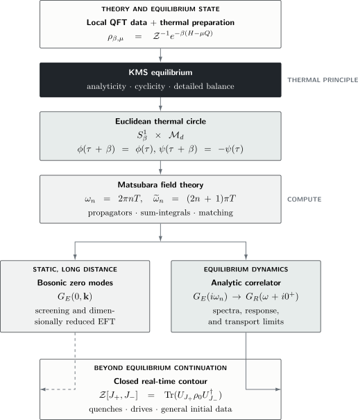
A thermal QFT begins with a state and an operator algebra. KMS equilibrium closes imaginary time into $S^1_\beta$, producing periodic bosonic and antiperiodic fermionic fields. Matsubara QFT then has two distinct exits: static zero modes can be matched to a lower-dimensional effective theory, while the common analytic correlator can be approached at real frequency to obtain retarded observables. General initial-value problems require a real-time contour rather than Euclidean continuation alone.

Spectral Data and Analytic Continuation

For a declared propagator convention, thermal Lehmann data define an analytic function away from the real axis. A common first-order convention is

$$\mathcal G(z,\mathbf k) = \int_{-\infty}^{\infty} dE\, \frac{ \rho(E,\mathbf k) }{ z-E }.$$

Its Matsubara values are samples at

$$z = i\zeta_n,$$

and its retarded boundary value is

$$\mathcal G^{\mathrm R}(E,\mathbf k) = \lim_{\epsilon\to0^+} \mathcal G(E+i\epsilon,\mathbf k).$$

The symbolic rule

$$i\zeta_n \longrightarrow E+i0^+$$

is therefore shorthand for identifying the correct analytic function and then taking its causal boundary value.

Relativistic scalar conventions illustrate why signs must be checked rather than guessed. The Euclidean denominator is

$$G_E(\omega_n,\mathbf k) = \frac1{ \omega_n^2+E_{\mathbf k}^2 },$$

while a common retarded convention is

$$G_R(\omega,\mathbf k) = \frac1{ \left( \omega+i0^+ \right)^2 -E_{\mathbf k}^2 }.$$

Consequently,

$$\begin{aligned} G_R(\omega,\mathbf k) &= - \left. G_E(\omega_n,\mathbf k) \right|_{\omega_n=\omega_n^\star}, \\ \omega_n^\star &= -i(\omega+i0^+) \end{aligned}$$

for these definitions. Other definitions can move the minus sign. The operator ordering, Fourier sign, Euclidean normalization, and spectral density must be fixed before any continuation rule is used.

Exact continuation is a statement about an analytic function with specified growth and spectral properties. Reconstructing that function from finitely many noisy Matsubara samples is an ill-conditioned inverse problem:

$$\begin{gathered} \text{finite noisy Matsubara data} \\ \not\Rightarrow \\ \text{a uniquely resolved spectrum} \end{gathered}$$

Baym–Mermin uniqueness for exact thermal data in the physical analytic class does not make finite numerical inversion well posed. Numerical claims need covariance, priors or regularization, sum rules, synthetic resolution tests, and uncertainty on features rather than only a smooth plotted curve.

Screening Is Not Real-Time Propagation

The static Euclidean correlator probes spatial screening:

$$G_E(0,\mathbf k) \simeq \frac{ Z_{\mathrm{scr}} }{ \mathbf k^2+m_{\mathrm{scr}}^2 }$$

near an isolated screening pole. In position space,

$$G_E(0,\mathbf x) \sim \frac{ e^{-m_{\mathrm{scr}}\lvert\mathbf x\rvert} }{ \lvert\mathbf x\rvert^{(d-1)/2} }$$

up to channel- and dimension-dependent powers.

A propagating excitation instead comes from a real-time pole or resonance:

$$G_R^{-1} \left( \omega_\star(\mathbf k), \mathbf k \right) = 0.$$

If the pole is weakly damped,

$$\omega_\star(\mathbf k) = \Omega_{\mathbf k} -i\Gamma_{\mathbf k}, \qquad \Gamma_{\mathbf k} \gt 0.$$

The quantities

$$m_{\mathrm{scr}}, \qquad \Omega_{\mathbf 0}, \qquad \Gamma_{\mathbf 0}$$

answer different questions. They can agree in a vacuum Lorentz-invariant limit, but a thermal medium does not require them to agree.

The order of limits can also matter:

$$\lim_{\omega\to0} \lim_{\mathbf k\to\mathbf0} \Pi(\omega,\mathbf k)$$

need not equal

$$\lim_{\mathbf k\to\mathbf0} \lim_{\omega\to0} \Pi(\omega,\mathbf k).$$

Static susceptibilities, uniform response, transport coefficients, and screening lengths should therefore be labeled by their limiting procedure.

Bosonic Zero Modes and Dimensional Reduction

The bosonic grid contains

$$\omega_0 = 0.$$

Every nonzero bosonic mode has

$$\lvert\omega_n\rvert \geq 2\pi T, \qquad n \ne 0,$$

while every thermal fermion mode has

$$\lvert\widetilde\omega_n\rvert \geq \pi T.$$

For static observables at spatial scales satisfying

$$\lvert\mathbf k\rvert \ll 2\pi T,$$

nonzero Matsubara modes may be integrated out. The remaining long-distance degrees of freedom are bosonic zero modes. Write

$$\phi(\tau,\mathbf x) = \phi_0(\mathbf x) + \phi_{\ne0}(\tau,\mathbf x).$$

After matching,

$$e^{-S_{\mathrm{eff}}[\phi_0]} = \int \mathcal D\phi_{\ne0}\, e^{-S_E[\phi_0+\phi_{\ne0}]}.$$

For the scalar example, the leading local form is

$$\begin{aligned} S_{\mathrm{eff}} &= \beta \int d^d x \left[ \frac12 \left( \boldsymbol\nabla\phi_0 \right)^2 \right. \\ &\qquad\left. + \frac12m_E^2\phi_0^2 + \frac{\lambda_E}{4!}\phi_0^4 + \cdots \right]. \end{aligned}$$

Defining a canonically normalized $d$-dimensional field,

$$\varphi := \sqrt{\beta}\, \phi_0,$$

gives

$$\begin{aligned} S_{\mathrm{eff}} &= \int d^d x \left[ \frac12 \left( \boldsymbol\nabla\varphi \right)^2 \right. \\ &\qquad\left. + \frac12m_E^2\varphi^2 + \frac{\lambda_d}{4!}\varphi^4 + \cdots \right], \end{aligned}$$

with tree-level matching

$$\lambda_d = \lambda T.$$

Loop matching changes the coefficients and generates every operator allowed by the symmetries. This is an effective field theory, not the instruction to delete all nonzero modes without calculation.

Dimensional reduction is useful when:

1. the target is static and long distance;
2. the nonzero modes are parametrically heavier than the retained scales;
3. matching can be controlled;
4. the reduced theory includes all relevant symmetry-allowed operators.

It can fail or require nonperturbative input when additional soft scales appear. Hot non-Abelian gauge theory is the standard warning: electric and magnetic sectors occur at different scales, and the deepest magnetic sector is intrinsically nonperturbative. Fermions lack a zero Matsubara mode, but they still affect the reduced theory through matching coefficients.

Statistical Field Theory Preview owns the classical field-distribution viewpoint, while Critical Phenomena and RG Bridge owns the scaling-limit and fixed-point translation.

Thermal Symmetry and Effective Potentials

Thermal fluctuations can change the curvature of an effective potential. For an order-parameter field,

$$V_{\mathrm{eff}}(\phi;T) = V_0(\phi) + \Delta V_T(\phi).$$

Near the origin one may define

$$m_{\mathrm{eff}}^2(T) := \left. \frac{ \partial^2V_{\mathrm{eff}} }{ \partial\phi^2 } \right|_{\phi=0}.$$

A sign change of this curvature can indicate a change in local stability:

$$m_{\mathrm{eff}}^2(T_c) = 0.$$

It does not by itself determine the order of the transition, the global minimum, the nucleation rate, or the reliability of perturbation theory. First-order transitions can occur before the curvature vanishes, while critical fluctuations can invalidate a low-order potential near a continuous transition.

Statements such as “temperature restores symmetry” are model dependent. Thermal restoration is common in weakly coupled scalar and gauge theories, but inverse symmetry breaking, nonrestoration, constraints, topology, and strong coupling can alter the conclusion.

Finite-Temperature Phase Transitions owns transition order, thermodynamic nonanalyticity, finite-size rounding, and critical diagnostics.

Chemical Potentials and Temporal Backgrounds

For a conserved charge,

$$\mathcal K = H-\mu Q.$$

In a charged Euclidean field theory, $\mu$ can often be represented as a constant imaginary temporal gauge potential. Schematically,

$$\partial_\tau \longrightarrow \partial_\tau-q\mu$$

for a field of charge $q$, with the precise sign determined by the charge and Euclidean-action conventions.

The effect is not simply a change in the occupation number. It shifts the quadratic kernel and can change stability. For a free relativistic charged boson, the grand-canonical ensemble requires the chemical potential to remain below the lowest charged excitation until condensation is treated explicitly.

For fermionic theories, a real chemical potential can make the Euclidean functional weight complex. Then

$$e^{-S_E} \notin \mathbb R_{\geq0}$$

configuration by configuration, even though the underlying thermal observable is well defined. This is the finite-density sign problem. It is a sampling obstruction, not evidence that the Hamiltonian theory is nonunitary.

Gauge Fields, Holonomy, and Static Sectors

Gauge fields are periodic around the thermal circle. A gauge transformation that is locally well behaved need not remove every constant temporal gauge field globally because the Euclidean time direction is compact.

The thermal holonomy is encoded by a Wilson line around the circle:

$$L(\mathbf x) = \mathcal P \exp \left[ ig \int_0^\beta d\tau\, A_0(\tau,\mathbf x) \right].$$

Its trace in a chosen representation is commonly called a Polyakov loop. Holonomy affects charged Matsubara modes and can serve as an order-parameter diagnostic in theories with an appropriate center symmetry.

Three cautions matter:

1. $A_0$ is not just another unconstrained scalar; gauge redundancy and Gauss-law constraints remain.
2. Gauge-dependent propagator poles are not automatically observable thermal masses.
3. A perturbative potential for the holonomy does not settle confinement or infrared magnetic dynamics in every regime.

These topics belong to dedicated thermal gauge theory rather than to this bridge, but the compact-circle geometry already explains why they arise.

Euclidean and Real-Time Questions

Different observables call for different formulations:

Question	Natural object	Main caution
pressure or equilibrium free energy	$\ln\mathcal Z$	vacuum subtraction and renormalization
static susceptibility	zero Matsubara mode	order of limits and conserved terms
screening length	spatial Euclidean correlator	not generally a pole mass
equilibrium spectrum	retarded boundary value	exact versus numerical continuation
transport coefficient	low-frequency retarded correlator	hydrodynamic limits and resummation
quench or driven evolution	closed-time-path correlators	KMS no longer closes the problem

For an equilibrium two-point function, Euclidean and retarded formulations can be boundary values of one analytic object. For higher-point functions, different real-time orderings correspond to different boundary regions and continuations. One naive replacement of every Matsubara frequency does not construct all real-time correlators.

For a genuinely time-dependent preparation, define a contour generating functional schematically as

$$\mathcal Z[J_+,J_-] = \operatorname{Tr} \left[ U_{J_+} \rho_0 U_{J_-}^{\dagger} \right].$$

The forward and backward sources are required to generate causal response, fluctuations, and occupations while preserving

$$\mathcal Z[J,J] = 1.$$

An imaginary contour segment can encode a correlated thermal initial state, but the real-time branches carry the subsequent dynamics.

Real-Time Thermal Dynamics Preview owns the greater, lesser, retarded, advanced, and Keldysh dictionary at the many-body level. The next QFT bridge develops why the closed time path is the natural continuation when equilibrium analytic continuation is no longer enough.

A Thermal QFT Workflow

1. Specify the state. Give $\beta$, chemical potentials, conserved charges, volume, and the thermodynamic limit.
2. Specify the observable. Distinguish free energy, Euclidean correlator, screening, spectral density, response, transport, and real-time evolution.
3. Choose the formulation. Use Euclidean time for equilibrium traces and static observables; use a real-time contour for general initial-value problems.
4. Declare conventions. Fix Fourier signs, thermal interval, Green-function normalization, and the generator $H-\mu Q$.
5. Identify the scales. Compare masses and external momenta with $T$, $2\pi T$, screening scales, and interaction scales.
6. Regulate before manipulating. Apply one ultraviolet regulator consistently to vacuum and thermal terms.
7. Separate vacuum and thermal pieces. Renormalize the former and test the convergence of the latter.
8. Resum or match when scales separate. A thermal mass inserted by hand is not a substitute for a controlled reorganization.
9. Continue only the analytic object. Do not continue a finite table by textual substitution.
10. Check exact constraints. Test KMS, periodicity, Ward identities, spectral sum rules, positivity where applicable, and limiting cases.

Common Mistakes

• Calling imaginary time physical time.
• Writing antiperiodic boundary conditions for every Grassmann field without checking its role in a thermal gauge-fixed theory.
• Mixing $\tau\in[0,\beta)$ with an explicit-$\hbar$ convention $\tau\in[0,\beta\hbar)$.
• Using a bosonic frequency on a fermion line or overlooking the bosonic parity of a fermion bilinear.
• Dropping the bosonic zero mode as if it were one negligible point in a continuum integral.
• Treating the Matsubara spacing $2\pi T$ as experimental real-frequency resolution.
• Replacing $i\omega_n$ by $\omega+i0^+$ before fixing the propagator convention and analytic class.
• Identifying a static screening mass with a real-time pole mass.
• Assuming the zero-temperature counterterms make every thermal perturbative expansion infrared safe.
• Integrating out nonzero modes without matching their effects into local operators.
• Treating the one-loop effective potential as exact near a strongly fluctuating phase transition.
• Assuming every stationary state satisfies KMS.
• Using equilibrium analytic continuation to describe a quench.
• Calling a gauge-dependent intermediate pole a measured quasiparticle without a gauge-invariant observable or controlled prescription.

Cross-Links

• Path Integrals for Many-Body Systems gives the operator-to-functional-integral bridge.
• Coherent-State Path Integrals develops bosonic and fermionic field variables from Fock space.
• Statistical Field Theory Preview separates thermal probability functionals from quantum amplitudes.
• Critical Phenomena and RG Bridge explains how a divergent correlation length defines continuum operator data and relevant deformations.
• Schwinger–Keldysh Bridge continues from equilibrium boundary values to doubled fields, initial states, response, noise, and nonequilibrium effective actions.
• Bridge to QFT places thermal methods within the wider route from quantum mechanics to fields.
• Continue on QFT.org records the publication status of the planned finite-temperature and finite-density destination and routes onward without a dead link.

References

1. T. Matsubara, “A New Approach to Quantum-Statistical Mechanics”, Progress of Theoretical Physics 14, 351–378 (1955).
2. P. C. Martin and J. Schwinger, “Theory of Many-Particle Systems. I”, Physical Review 115, 1342–1373 (1959).
3. R. Kubo, “Statistical-Mechanical Theory of Irreversible Processes. I”, Journal of the Physical Society of Japan 12, 570–586 (1957).
4. G. Baym and N. D. Mermin, “Determination of Thermodynamic Green’s Functions”, Journal of Mathematical Physics 2, 232–234 (1961).
5. R. Haag, N. M. Hugenholtz, and M. Winnink, “On the Equilibrium States in Quantum Statistical Mechanics”, Communications in Mathematical Physics 5, 215–236 (1967).
6. L. Dolan and R. Jackiw, “Symmetry Behavior at Finite Temperature”, Physical Review D 9, 3320–3341 (1974).
7. S. Weinberg, “Gauge and Global Symmetries at High Temperature”, Physical Review D 9, 3357–3378 (1974).
8. A. D. Linde, “Infrared Problem in Thermodynamics of the Yang–Mills Gas”, Physics Letters B 96, 289–292 (1980).
9. T. Appelquist and R. D. Pisarski, “High-Temperature Yang–Mills Theories and Three-Dimensional Quantum Chromodynamics”, Physical Review D 23, 2305–2317 (1981).
10. N. P. Landsman and Ch. G. van Weert, “Real- and Imaginary-Time Field Theory at Finite Temperature and Density”, Physics Reports 145, 141–249 (1987).
11. M. Le Bellac, Thermal Field Theory, Cambridge University Press (1996).
12. J. I. Kapusta and C. Gale, Finite-Temperature Field Theory: Principles and Applications, 2nd ed., Cambridge University Press (2006).

Exercises

1. Derive the thermal frequency grids

Let

$$f(\tau) = e^{i\omega\tau}.$$

Derive the allowed $\omega$ for periodic and antiperiodic fields on a circle of circumference $\beta$. Explain why a fermion bilinear has bosonic external frequency.

Solution

Periodicity requires

$$e^{i\omega(\tau+\beta)} = e^{i\omega\tau},$$

so

$$e^{i\omega\beta} = 1.$$

Therefore

$$\omega = \omega_n = 2\pi nT, \qquad n\in\mathbb Z.$$

Antiperiodicity requires

$$e^{i\omega\beta} = -1,$$

which gives

$$\omega = \widetilde\omega_n = (2n+1)\pi T.$$

A bilinear contains two odd fields and therefore has even fermion parity. In frequency arithmetic,

$$\widetilde\omega_n -\widetilde\omega_m = 2\pi(n-m)T,$$

which lies on the bosonic grid. Density, current, and pair susceptibilities therefore carry bosonic external Matsubara frequency even when their internal lines are fermionic.

2. Check the free scalar thermal propagator

Starting from

$$\begin{aligned} G_E(\tau,\mathbf k) &= \frac1{2E_{\mathbf k}} \left[ \left( 1+n_{\mathrm B} \right) e^{-E_{\mathbf k}\tau} \right. \\ &\qquad\left. + n_{\mathrm B} e^{E_{\mathbf k}\tau} \right], \end{aligned}$$

show that it is periodic and symmetric under

$$\tau \longmapsto \beta-\tau.$$

Then evaluate $G_E(0,\mathbf k)$.

Solution

The Bose factor satisfies

$$1+n_{\mathrm B}(E) = e^{\beta E} n_{\mathrm B}(E).$$

Using this identity,

$$\begin{aligned} G_E(\beta-\tau,\mathbf k) &= \frac1{2E_{\mathbf k}} \Bigl[ n_{\mathrm B} e^{E_{\mathbf k}\tau} \\ &\qquad+ \left( 1+n_{\mathrm B} \right) e^{-E_{\mathbf k}\tau} \Bigr] \\ &= G_E(\tau,\mathbf k). \end{aligned}$$

Extending by the same thermal boundary relation gives

$$G_E(\tau+\beta,\mathbf k) = G_E(\tau,\mathbf k).$$

At $\tau=0$,

$$\begin{aligned} G_E(0,\mathbf k) &= \frac1{2E_{\mathbf k}} \left[ 1 + 2n_{\mathrm B}(E_{\mathbf k}) \right]. \end{aligned}$$

The $1/(2E_{\mathbf k})$ term survives at zero temperature, while the $n_{\mathrm B}/E_{\mathbf k}$ term is thermal.

3. Derive the scalar thermal mass

For massless $\lambda\phi^4/4!$ theory in three spatial dimensions, evaluate

$$\Pi_{\mathrm{th}}(T) = \frac{\lambda}{2} \int \frac{d^3k}{(2\pi)^3} \frac{ n_{\mathrm B}(k) }{ k }.$$

You may use

$$\int_0^\infty dx\, \frac{x}{e^x-1} = \frac{\pi^2}{6}.$$

Solution

Spherical symmetry gives

$$\begin{aligned} \int \frac{d^3k}{(2\pi)^3} \frac{ n_{\mathrm B}(k) }{ k } &= \frac1{2\pi^2} \int_0^\infty dk\, \frac{k}{e^{\beta k}-1}. \end{aligned}$$

Set $x=\beta k$. Then

$$\begin{aligned} \int \frac{d^3k}{(2\pi)^3} \frac{ n_{\mathrm B}(k) }{ k } &= \frac{T^2}{2\pi^2} \int_0^\infty dx\, \frac{x}{e^x-1} \\ &= \frac{T^2}{12}. \end{aligned}$$

Therefore

$$\Pi_{\mathrm{th}}(T) = \frac{\lambda T^2}{24}.$$

The result is the leading one-loop thermal self-energy in this convention. It does not prove that an unreorganized loop expansion remains accurate when the induced scale controls the infrared.

4. Canonically normalize the zero mode

Suppose a four-dimensional scalar theory has a static action

$$\begin{aligned} S_0 &= \beta \int d^3x \left[ \frac12 \left( \boldsymbol\nabla\phi_0 \right)^2 \right. \\ &\qquad\left. + \frac12m_E^2\phi_0^2 + \frac{\lambda}{4!}\phi_0^4 \right]. \end{aligned}$$

Find the canonically normalized three-dimensional field and the tree-level three-dimensional quartic coupling.

Solution

Define

$$\varphi = \sqrt{\beta}\, \phi_0.$$

Then

$$\phi_0 = \sqrt{T}\, \varphi.$$

The gradient term becomes

$$\beta \frac12 \left( \boldsymbol\nabla\phi_0 \right)^2 = \frac12 \left( \boldsymbol\nabla\varphi \right)^2.$$

The quartic term becomes

$$\beta \frac{\lambda}{4!} \phi_0^4 = \frac{\lambda T}{4!} \varphi^4.$$

Thus

$$\lambda_3 = \lambda T$$

at tree level. Integrating out nonzero Matsubara modes shifts $m_E^2$, $\lambda_3$, and higher-operator coefficients.

5. Continue a free scalar propagator

Using the conventions

$$G_E(\omega_n,\mathbf k) = \frac1{ \omega_n^2+E_{\mathbf k}^2 }$$

and

$$G_R(\omega,\mathbf k) = \frac1{ \left( \omega+i0^+ \right)^2 -E_{\mathbf k}^2 },$$

show the continuation relation between them and locate the retarded poles.

Solution

Make the replacement

$$\omega_n \longrightarrow -i \left( \omega+i0^+ \right).$$

Then

Define

$$\omega_n^\star = -i(\omega+i0^+).$$

Then

$$\left( \omega_n^\star \right)^2 + E_{\mathbf k}^2 = E_{\mathbf k}^2 - \left( \omega+i0^+ \right)^2,$$

and therefore

$$G_E \left( \omega_n^\star, \mathbf k \right) = - G_R(\omega,\mathbf k).$$

Hence

$$G_R = - G_E \left( \omega_n \to -i(\omega+i0^+) \right)$$

for these definitions. The poles lie infinitesimally below the real axis at

$$\omega = \pm E_{\mathbf k} -i0^+.$$

The overall minus sign is convention dependent; the retarded half-plane placement is physical.

6. Distinguish screening and pole masses

Suppose the inverse propagators are

$$G_E^{-1}(0,\mathbf k) = \mathbf k^2+m^2+\Pi_E(0,\mathbf k)$$

and

$$G_R^{-1}(\omega,\mathbf0) = \omega^2-m^2-\Pi_R(\omega,\mathbf0).$$

Write the equations defining a static screening mass and a zero-momentum pole energy. Under what special condition must they agree?

Solution

A screening pole occurs after continuing spatial momentum to

$$\mathbf k^2 = -m_{\mathrm{scr}}^2.$$

It satisfies

$$-m_{\mathrm{scr}}^2 +m^2 + \Pi_E \left( 0, \mathbf k^2=-m_{\mathrm{scr}}^2 \right) = 0.$$

The real-time pole energy satisfies

$$\Omega_{\mathbf0}^2 -m^2 - \operatorname{Re} \Pi_R(\Omega_{\mathbf0},\mathbf0) = 0,$$

with the imaginary part determining damping when a narrow pole exists.

The two equations sample different kinematics. They are forced to agree in a Lorentz-invariant vacuum when the self-energy depends only on

$$p^2 = \omega^2-\mathbf k^2$$

and both definitions identify the same isolated stable pole. A thermal state breaks boost invariance, so no general equality remains.

7. Recover detailed balance from KMS

Assume

$$C^>(t) = C^<(t+i\beta)$$

and

$$\widetilde C(\omega) = \int_{-\infty}^{\infty} dt\, e^{i\omega t} C(t).$$

Derive the frequency-domain detailed-balance relation. State the analytic assumption used.

Solution

Insert the KMS relation:

$$\widetilde C^>(\omega) = \int_{-\infty}^{\infty} dt\, e^{i\omega t} C^<(t+i\beta).$$

Set

$$z = t+i\beta.$$

Then

$$e^{i\omega t} = e^{i\omega z} e^{\beta\omega}.$$

If $C^<(z)$ is analytic in the thermal strip and decays sufficiently to move the contour back to the real axis without endpoint contributions,

$$\widetilde C^>(\omega) = e^{\beta\omega} \widetilde C^<(\omega).$$

Therefore

$$\widetilde C^<(\omega) = e^{-\beta\omega} \widetilde C^>(\omega).$$

Changing the Fourier sign or the definition of the lesser correlator changes the displayed placement of signs, so those conventions belong to the result.

8. Choose the right thermal formulation

Choose the smallest adequate formulation for each task:

1. the pressure of an equilibrium scalar plasma;
2. a spatial screening length;
3. an equilibrium spectral peak from exact analytic data;
4. a conductivity;
5. the occupation dynamics after a sudden quench.

Explain each choice and one major caveat.

Solution

1. The pressure follows from the equilibrium partition function,

   $$P = \frac{T}{V} \ln\mathcal Z,$$

   so Euclidean thermal QFT is natural. Vacuum subtraction, renormalization, and infrared resummation may be required.

2. A spatial screening length comes from a static Euclidean correlator or the zero Matsubara sector. It should not be labeled a real-time pole mass.

3. Exact analytic thermal data can define the common spectral function and its retarded boundary value. With finite noisy data, continuation becomes an inverse problem and the attainable resolution must be demonstrated.

4. Conductivity is a low-frequency retarded response coefficient. An equilibrium Euclidean calculation may provide input, but analytic continuation, the order of limits, Ward identities, and often ladder or kinetic resummation are central.

5. A quench is an initial-value problem. A Schwinger–Keldysh or another explicit real-time method is required because a single equilibrium KMS state does not determine the evolving occupations.