Finite-Temperature Phase Transitions

A finite-temperature phase transition is a sharp change of equilibrium phase that occurs when temperature or another thermodynamic control crosses a phase boundary at nonzero temperature.

For a finite system of linear size $L$, define

$$\begin{aligned} Z_L(T,\boldsymbol\lambda) &:= \operatorname{Tr} e^{-\beta H_L(\boldsymbol\lambda)}, \\ \beta &:= \frac{1}{k_{\mathrm B}T}. \end{aligned}$$

and the free-energy density

$$f_L(T,\boldsymbol\lambda) := -\frac{k_{\mathrm B}T}{V_L} \ln Z_L(T,\boldsymbol\lambda).$$

Here $\boldsymbol\lambda$ denotes fields, pressure proxies, chemical potentials, couplings, or other controls, and $V_L$ is the volume or number of unit cells used to normalize extensive quantities.

The sharp transition belongs to the bulk limit

$$f(T,\boldsymbol\lambda) := \lim_{L\to\infty} f_L(T,\boldsymbol\lambda).$$

At a phase boundary, this limiting thermodynamic potential is nonanalytic in at least one physical control. A finite sample usually replaces the singularity by a rounded crossover.

The central distinction is:

Transition	Bulk signature	Typical finite-size precursor
first order	coexisting phases and a first-derivative jump	bimodal distributions
continuous	diverging length scale and singular response	growing, narrowing peaks

These are equilibrium classifications. Hysteresis, slow relaxation, or a dramatic finite-size peak can support an interpretation, but none is the definition by itself.

Canonical Scope

This page is the canonical home for:

• thermal phase boundaries as nonanalyticities of bulk thermodynamic potentials;
• why ordinary finite systems are analytic and transitions are rounded;
• critical temperature and reduced-temperature conventions;
• first-order coexistence, latent heat, and discontinuous conjugate densities;
• continuous transitions, correlation-length growth, and critical fluctuations;
• a preview of ordinary finite-size scaling for both transition types;
• Lee–Yang and Fisher zeros as a mechanism for bulk singularity;
• the role of quantum mechanics at nonzero temperature;
• symmetry, dimensionality, and interaction-range restrictions;
• numerical and experimental evidence standards.

Neighboring pages retain separate ownership:

• Thermodynamic Potentials owns Legendre transforms, natural variables, stability, coexistence conditions, and the Clapeyron equation.
• Fluctuations and Susceptibilities owns exact equilibrium covariance identities and their quantum Kubo–Mori form.
• Order Parameters owns operator definitions, source conventions, and finite-size estimators.
• Spontaneous Symmetry Breaking owns pure-phase selection, symmetry-restored finite states, and noncommuting source and volume limits.
• Landau Theory owns uniform analytic order-parameter potentials, their minima, mean-field exponents, polynomial coexistence, and tricriticality.
• Landau–Ginzburg Theory Preview owns the static spatial functional, Gaussian correlation length, interfaces, and the Ginzburg criterion.
• Long-Range Order owns correlation limits and Bragg-peak scaling.
• Quantum Phase Transitions owns zero-temperature parameter-driven transitions, quantum-critical fans, and imaginary-time scaling at $T=0$.
• The later Critical Exponents and Scaling page owns exponent identities, data collapse, corrections to scaling, and dynamic scaling in depth.
• Model pages retain exact phase diagrams, critical temperatures, spectra, and microscopic observables.

The purpose here is to decide whether a nonzero-temperature boundary exists, what kind it is, and what finite evidence can support that conclusion.

Equilibrium Setup

The thermodynamic potential must match the controls.

Fixed particle number and volume

In the canonical ensemble,

$$F_L(T,V,N) := -k_{\mathrm B}T \ln Z_{L,N}(T,V).$$

The natural intensive bulk quantity is

$$\begin{aligned} f(T,n) &:= \lim_{V\to\infty} \frac{F(T,V,N)}{V}, \\ n &:= \frac{N}{V}. \end{aligned}$$

The limit holds $n$ and the sample shape or aspect-ratio sequence fixed.

Fixed chemical potential

In the grand-canonical ensemble,

$$\mathcal Z_L(T,V,\mu) := \operatorname{Tr} \exp \left[ -\beta \left( H_L-\mu N_L \right) \right],$$

with grand-potential density

$$\omega(T,\mu) := \lim_{V\to\infty} \left[ -\frac{k_{\mathrm B}T}{V} \ln\mathcal Z_L \right].$$

A density jump is a first derivative of $\omega$, while a phase-separated canonical state can occupy a density interval at the same coexistence chemical potential. The two descriptions are related, but finite-size histograms and constraints need not look identical.

Source convention

For an ordering operator $M_L$ and source $h$,

$$H_L(h) := H_L(0)-hM_L.$$

The intensive conjugate variable is

$$m := -\frac{\partial f}{\partial h}.$$

One must state whether $h$ is set to zero before or after the bulk limit. At a symmetry-breaking transition, those orders of limits distinguish a symmetric mixture from a selected ordered phase.

Why Finite Systems Are Usually Analytic

For a finite-dimensional Hilbert space with finite energies $E_{n,L}$,

$$Z_L(\beta) := \sum_{n=1}^{D_L} e^{-\beta E_{n,L}}.$$

Every term is analytic in $\beta$, and for real $\beta\gt0$,

$$Z_L(\beta) \gt 0.$$

Therefore

$$F_L(\beta) := -\beta^{-1} \ln Z_L(\beta)$$

is analytic at every positive real temperature, provided the Hamiltonian depends regularly on the other controls.

For an infinite-dimensional Hilbert space, the corresponding statement requires

$$e^{-\beta H_L}$$

to be trace class in the temperature interval of interest. A divergent finite-volume partition function signals a different mathematical problem, not an ordinary many-body phase transition.

Analyticity does not mean that finite curves must look gentle. If $V_L$ is large, a rounded change can be extremely steep. The distinction is exact:

$$\begin{aligned} L<\infty &: \quad \text{analytic}, \\ L\to\infty &: \quad \text{nonanalyticity possible}. \end{aligned}$$

An isolated finite-level crossing can create a nonanalytic zero-temperature ground-state energy. At $T\gt0$, the trace generally sums both levels smoothly. That is another reason not to infer a thermal bulk transition from one small spectrum.

How the Bulk Limit Becomes Singular

The number of many-body states grows exponentially with volume. Their competition can leave an order-one imprint on the free-energy density even though each finite partition function is analytic.

Suppose

$$Z_L \simeq e^{-\beta V_L f_A} + e^{-\beta V_L f_B}.$$

Then

$$f_L \simeq -\frac{k_{\mathrm B}T}{V_L} \ln \left[ e^{-\beta V_L f_A} + e^{-\beta V_L f_B} \right].$$

As $V_L\to\infty$,

$$f_L \longrightarrow \min \left( f_A,f_B \right).$$

The minimum of two analytic branches can have a cusp where the branches exchange stability. The logarithm smooths that cusp at finite size over a window that shrinks with volume.

This mechanism is not limited to two phases. More generally, singularity appears when an exponentially large state count, diverging correlation volume, or competing thermodynamic saddle defeats uniform analyticity of the finite-size sequence.

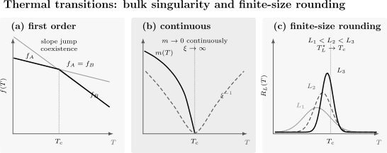
Three complementary signatures. At an ordinary first-order transition, two analytic free-energy branches exchange stability and the lower envelope develops a cusp. At a conventional continuous transition, the order parameter can vanish continuously while the inverse correlation length tends to zero. Every finite system remains rounded; response peaks sharpen and their pseudocritical locations $T_L^\star$ approach the bulk $T_c$ only along a controlled size sequence.

First-Order Transitions

A first-order transition has coexistence of distinct equilibrium phases and a discontinuity in at least one first derivative of the appropriate bulk thermodynamic potential.

At fixed volume and source, define the entropy density

$$s := -\left( \frac{\partial f}{\partial T} \right)_h$$

and the conjugate order density

$$m := -\left( \frac{\partial f}{\partial h} \right)_T.$$

At coexistence,

$$f_A(T_c,h_c) := f_B(T_c,h_c),$$

but one or both derivatives can differ:

$$\Delta s := s_B-s_A \ne 0,$$

or

$$\Delta m := m_B-m_A \ne 0.$$

Latent heat

The latent-heat density is

$$\ell := T_c\Delta s.$$

Because

$$e := f+Ts,$$

equality of $f_A$ and $f_B$ at coexistence gives

$$\Delta e := e_B-e_A := T_c\Delta s := \ell.$$

The sign depends on the order in which the phases are subtracted. The physically reported latent heat is usually its positive magnitude for the stated heating or cooling process.

Thermodynamic Potentials develops coexistence under pressure and the Clapeyron relation. This page uses only the local transition signatures.

Coexistence

At $T_c$, macroscopic regions of both phases can coexist. For short-range interactions, an interface carries a free-energy cost that commonly scales as

$$\Delta F_{\mathrm{int}} \sim \sigma L^{d-1},$$

where $\sigma$ is an orientation-dependent interface tension.

Under periodic boundary conditions, a slab configuration can contain two interfaces, changing the coefficient but not the area scaling. Open boundaries, wetting, anisotropy, long-range forces, and conserved quantities can alter the finite geometry.

Probability distributions

For an intensive order parameter $m_L=M_L/V_L$, a finite coexistence distribution often has two peaks:

$$P_L(m) \simeq w_A P_{A,L}(m) + w_B P_{B,L}(m).$$

The peaks approach the bulk phase values $m_A$ and $m_B$. The probability minimum between them is controlled by interface configurations and sampling dynamics.

A bimodal histogram is strong evidence only when:

• both peaks stabilize under increasing size;
• the valley deepens consistently with an interface cost;
• the relative weights are interpreted with the correct phase degeneracies;
• the simulation or experiment tunnels enough to sample both phases;
• boundary conditions are reported.

Two peaks in a noisy or poorly equilibrated small sample are not sufficient.

Metastability and hysteresis

A local free-energy minimum can persist beyond coexistence as a metastable state. Sweeping temperature then produces history dependence and hysteresis.

Hysteresis is not the equilibrium definition of first order:

• a genuine first-order transition may show little hysteresis under slow equilibration or efficient nucleation;
• kinetic arrest can produce hysteresis without an equilibrium phase boundary;
• the observed loop depends on sweep rate, disorder, defects, and coupling to the environment.

Equilibrium coexistence, latent heat, distributions, and size scaling must be separated from protocol-dependent kinetics.

Continuous Transitions

A continuous transition has no coexistence jump in the order parameter or entropy density along the transition path, but the bulk state becomes nonanalytic through long-range fluctuations.

For a conventional symmetry-breaking transition,

$$\lim_{T\to T_c^-} m(T) := 0,$$

while

$$\Delta s := 0.$$

The specific-heat density is

$$c_h := -T \left( \frac{\partial^2 f}{\partial T^2} \right)_h,$$

and the static susceptibility is

$$\chi_T := -\left( \frac{\partial^2 f}{\partial h^2} \right)_T.$$

Either can diverge, develop a cusp, remain finite with a singular derivative, or mix with other observables. A continuous transition does not require every response to diverge.

Why the Ehrenfest label is insufficient

The historical Ehrenfest scheme classified transitions by the lowest discontinuous derivative of a thermodynamic potential. Modern work usually emphasizes:

• first order, with phase coexistence and first-derivative jumps;
• continuous, with a diverging length scale or other critical singularity;
• transitions outside the ordinary power-law pattern, such as Berezinskii–Kosterlitz–Thouless transitions.

The derivative-order label can fail when a singularity is logarithmic, essential, extremely weak, or not naturally described by a local order parameter.

Critical Temperature

The critical temperature $T_c$ is the bulk temperature at a continuous transition or critical endpoint. For a first-order line, the more precise term is often transition temperature or coexistence temperature, though $T_c$ is also used in practice.

Define the reduced temperature

$$t := \frac{T-T_c}{T_c}.$$

Then

$$t\lt0$$

is below $T_c$, while

$$t\gt0$$

is above it.

The value of $T_c$ is nonuniversal. It can depend on:

• microscopic couplings and density;
• dimensionality and lattice geometry;
• interaction range and anisotropy;
• pressure, field, chemical potential, or disorder;
• the ensemble and thermodynamic path;
• whether the system is uniform, trapped, layered, or finite.

A system can have several transitions, reentrant order, a critical endpoint, or no nonzero $T_c$ at all. A fitted temperature scale should not be called $T_c$ until size or bulk evidence distinguishes a singular boundary from a crossover.

Correlation Length and Critical Fluctuations

For a local ordering field $\phi(\mathbf r)$, define the connected equilibrium correlator

$$G_c(\mathbf r) := \left\langle \phi(\mathbf r)\phi(\mathbf0) \right\rangle - \left\langle \phi(\mathbf r) \right\rangle \left\langle \phi(\mathbf0) \right\rangle.$$

Away from criticality, a short-range phase commonly has

$$G_c(r) \sim \frac{e^{-r/\xi}}{r^p}$$

at large $r$, with a finite correlation length $\xi$ and a model-dependent algebraic prefactor.

Near an ordinary continuous transition,

$$\xi(t) \sim \xi_\pm \lvert t\rvert^{-\nu},$$

where the amplitudes above and below $T_c$ need not be equal.

At scales

$$a \ll r \ll \xi,$$

a common critical form is

$$G_c(r) \sim \frac{1}{ r^{d-2+\eta} }.$$

Consequently, a susceptibility coupled to the same channel scales schematically as

$$\chi \propto \int^{\xi} d^dr\, G_c(r) \sim \xi^{2-\eta},$$

provided the source normalization, conservation laws, and ensemble match the stated response.

The growing correlation volume

$$V_\xi \sim \xi^d$$

contains increasingly coherent fluctuations. Ordinary independent-block or central-limit intuition fails when $\xi$ becomes comparable with the sample size.

Connected Correlation Functions owns the subtraction and clustering conventions. Fluctuations and Susceptibilities owns the exact integrated-correlation and Kubo–Mori response identities.

A Preview of Critical Exponents

Power-law criticality is often summarized by

$$\begin{aligned} \xi &\sim \lvert t\rvert^{-\nu}, \\ m &\sim (-t)^{\beta_{\mathrm{op}}}, \qquad t\to0^-, \\ \chi &\sim \lvert t\rvert^{-\gamma}, \\ c_h^{\mathrm{sing}} &\sim \lvert t\rvert^{-\alpha}. \end{aligned}$$

The subscript on $\beta_{\mathrm{op}}$ distinguishes the order-parameter exponent from inverse temperature.

These formulas are a preview, not a license to fit four independent straight lines. Critical Exponents and Scaling owns:

• scaling functions and exponent identities;
• upper critical dimensions;
• dangerously irrelevant variables;
• analytic backgrounds and corrections to scaling;
• anisotropic and dynamic exponents;
• covariance-aware data collapse.

Here the operational lesson is simpler: continuous criticality must be established through a consistent long-distance and finite-size pattern, not one apparent power law.

Finite-Size Rounding

A finite sample cannot support

$$\xi \to \infty.$$

The size $L$ becomes an infrared cutoff. A measured or computed peak therefore occurs at a pseudocritical temperature

$$T_L^\star,$$

defined by a stated criterion such as:

• a susceptibility maximum;
• a heat-capacity maximum;
• a Binder-ratio crossing;
• a correlation-length-ratio crossing;
• equal phase weights;
• equal peak heights.

Different criteria need not agree at finite $L$. A valid transition estimate requires

$$\lim_{L\to\infty} T_L^\star := T_c$$

with a controlled extrapolation.

Continuous-transition scaling preview

For an ordinary continuous transition, a singular free-energy density often has the finite-size form

$$f_{s,L}(t,h) := L^{-d} \mathcal F \left( tL^{1/\nu}, hL^{y_h} \right),$$

up to aspect-ratio, boundary, and correction-to-scaling terms.

This suggests a rounding width

$$\delta t_L \sim L^{-1/\nu}$$

and, under the corresponding scaling hypotheses,

$$\chi_L^{\max} \sim L^{\gamma/\nu}.$$

Dimensionless ratios can approach size-independent critical values, but crossings drift when irrelevant fields, boundaries, or anisotropy matter.

Binder ratio

For a scalar, symmetry-centered order parameter,

$$U_{4,L} := 1 - \frac{ \left\langle m_L^4\right\rangle }{ 3 \left\langle m_L^2\right\rangle^2 }.$$

The factor $3$ is conventional and changes for vector order parameters or alternative cumulant definitions. Near a continuous transition, curves for different sizes can cross close to $T_c$. Near coexistence, non-Gaussian or bimodal distributions can produce very different behavior.

Quoting a Binder number without its definition, boundary conditions, and order-parameter normalization is not reproducible.

Two-Phase Model for First-Order Rounding

Let phases $A$ and $B$ have degeneracies $g_A$ and $g_B$. A minimal finite-volume partition function is

$$Z_L \simeq g_A e^{-\beta V_L f_A} + g_B e^{-\beta V_L f_B}.$$

Define

$$x := \beta V_L \left( f_B-f_A \right) - \ln \left( \frac{g_B}{g_A} \right).$$

Then

$$w_B := \frac{1}{1+e^x}, \qquad w_A := 1-w_B.$$

Near coexistence,

$$f_B-f_A \simeq -\Delta s \left( T-T_c \right).$$

Changing $w_B$ by an order-one amount requires

$$\lvert x\rvert \sim 1.$$

Therefore the ordinary rounding width scales as

$$\delta T_L \sim V_L^{-1} \sim L^{-d}.$$

At equal weights and neglecting within-phase fluctuations,

$$\operatorname{Var}(E) \simeq \frac{ V_L^2 \left( \Delta e \right)^2 }{4}.$$

Since

$$C_V := \frac{ \operatorname{Var}(E) }{ k_{\mathrm B}T^2 },$$

the specific heat per volume satisfies

$$\left( \frac{C_V}{V_L} \right)_{\max} \simeq \frac{ V_L \left( \Delta e \right)^2 }{ 4k_{\mathrm B}T_c^2 }.$$

Thus an ordinary first-order peak in $C_V/V_L$ grows proportionally to volume.

The same logic gives, for an order parameter with phase jump $\Delta m$,

$$\chi_L^{\max} \propto V_L \left( \Delta m \right)^2.$$

These are asymptotic statements, not universal small-size fitting laws. Boundary conditions, interfacial terms, constrained ensembles, disorder, and degeneracies that grow with $L$ can change leading shifts or produce nonstandard scaling.

Complex Zeros and Real Singularities

Finite partition functions can be understood through their zeros in a complexified control.

Let $z$ be a fugacity, field variable, or temperature-like parameter such that

$$Z_L(z) := C_L \prod_{j=1}^{N_L} \left( z-z_{j,L} \right).$$

At finite size, the zeros $z_{j,L}$ avoid the physical region where $Z_L$ is positive. The free-energy density contains

$$\begin{aligned} f_L(z) &= -\frac{k_{\mathrm B}T}{V_L} \ln C_L \\ &\quad -\frac{k_{\mathrm B}T}{V_L} \sum_j \ln \left( z-z_{j,L} \right). \end{aligned}$$

A sequence of zeros can approach or pinch the physical axis as $L\to\infty$. Their accumulation then obstructs analytic continuation and produces a bulk singularity.

Lee–Yang zeros

Lee–Yang zeros complexify fugacity or magnetic field. For the ferromagnetic Ising model, the circle theorem constrains their location in an appropriate complex fugacity variable. Their approach to the real physical axis encodes field-driven nonanalyticity.

Fisher zeros

Fisher zeros complexify temperature or inverse temperature. Their closest distance to the real axis and their approach angle contain finite-size and critical information.

Complex zeros are not additional phases. They are a diagnostic language for how an analytic finite sequence develops a nonanalytic bulk limit.

Quantum Mechanics at Nonzero Temperature

A thermal transition in a quantum many-body system is not “classical” merely because $T\gt0$. The Gibbs operator still contains the full quantum Hamiltonian:

$$\rho_\beta := \frac{e^{-\beta H}}{Z}.$$

Noncommuting terms determine:

• the spectrum and matrix elements;
• effective interactions among thermal degrees of freedom;
• the value of $T_c$;
• the order-parameter structure;
• topological defects and collective modes;
• which low-energy fields survive coarse graining.

Why classical critical behavior often emerges

In an equilibrium imaginary-time formulation, bosonic fields are periodic on a circle of length

$$\beta\hbar.$$

Their Matsubara frequencies are

$$\omega_n := \frac{2\pi n}{\beta\hbar}.$$

At a nonzero-temperature continuous transition, the bosonic zero-frequency mode can become critical, while nonzero modes retain a frequency scale of order

$$\frac{2\pi k_{\mathrm B}T}{\hbar}.$$

When the nonzero modes can be integrated out locally, the longest-distance static singularity is governed by an effective $d$-dimensional classical field theory.

This dimensional-reduction intuition has conditions. Gapless fermions, gauge fields, long-range interactions, disorder, constraints, or additional soft modes can generate nonlocal or otherwise modified effective theories.

Finite-Temperature QM Overview owns the operator, imaginary-time, Matsubara, and spectral toolkit.

Thermal versus quantum criticality

A thermal critical point occurs at

$$T_c \gt 0.$$

A quantum critical point occurs at

$$T := 0$$

as a nonthermal Hamiltonian parameter is tuned.

A quantum critical point can organize finite-temperature crossovers, but a crossover line in a quantum-critical fan is not automatically a thermal phase boundary. Conversely, a finite-temperature ordered phase can terminate at a genuine thermal transition above a zero-temperature phase.

Symmetry, Dimension, and Interaction Range

The existence of $T_c$ is constrained by more than the local Hamiltonian.

Discrete symmetry

Short-range one-dimensional Ising order is destroyed at every $T\gt0$ by a finite density of domain walls. In two dimensions, the square-lattice Ising model has a genuine nonzero-temperature transition.

Discrete symmetry alone does not guarantee a transition in every dimension or geometry. Connectivity, disorder, frustration, and interaction range still matter.

Continuous symmetry

For one- and two-dimensional isotropic Heisenberg models with finite-range exchange, the Mermin–Wagner theorem excludes ordinary ferromagnetic or antiferromagnetic long-range order at nonzero temperature.

The assumptions matter:

• continuous symmetry;
• sufficiently short-range interactions;
• low spatial dimension;
• the relevant equilibrium setting.

Easy-axis anisotropy, interlayer coupling, long-range interactions, or explicit fields can change the conclusion.

Two-dimensional topological transition

A two-dimensional system can undergo a Berezinskii–Kosterlitz–Thouless transition even though ordinary continuous-symmetry long-range order remains absent.

Above the transition, the correlation length has an essential singularity of the form

$$\xi \sim \xi_0 \exp \left( \frac{b}{\sqrt{t}} \right), \qquad t\to0^+.$$

Below the transition, correlations are algebraic rather than asymptoting to a nonzero local order parameter. This is a primary counterexample to classifying every continuous transition by a simple power-law order parameter.

Long-range and nonadditive systems

Interactions that decay too slowly can change:

• the existence and value of $T_c$;
• critical exponents;
• additivity and ensemble equivalence;
• interface scaling;
• the shape of finite-size rounding.

The interaction kernel and thermodynamic normalization must be stated before short-range finite-size laws are applied.

Benchmark: One-Dimensional Ising Correlations

Consider the diagonal quantum-spin Hamiltonian

$$H_L := -J \sum_{j=1}^{L} \sigma_j^z \sigma_{j+1}^z, \qquad J\gt0.$$

Because all terms commute, its thermal statistics are those of the classical one-dimensional Ising chain.

At zero field in the infinite chain,

$$\left\langle \sigma_0^z \sigma_r^z \right\rangle := \left[ \tanh \left( \beta J \right) \right]^r.$$

Writing this as

$$\left\langle \sigma_0^z \sigma_r^z \right\rangle := e^{-ra/\xi}$$

gives

$$\xi^{-1} := -\frac{1}{a} \ln \left[ \tanh \left( \beta J \right) \right].$$

For every finite $T$,

$$0 \lt \tanh(\beta J) \lt 1,$$

so $\xi$ is finite. It grows exponentially at low temperature:

$$\xi \sim \frac{a}{2} e^{2\beta J}.$$

A chain with

$$L \ll \frac{\xi}{a}$$

can look nearly ordered, yet its apparent threshold drifts toward $T=0$ as $L$ increases. This is finite-size crossover, not a nonzero bulk $T_c$.

The Transverse-Field Ising Model adds noncommuting quantum fluctuations and has a zero-temperature critical point, but its short-range one-dimensional form still has no nonzero-temperature Ising-ordering transition.

Benchmark: Square-Lattice Ising Criticality

For the two-dimensional nearest-neighbor ferromagnetic Ising model at zero field, the exact critical coupling satisfies

$$\sinh \left( \frac{2J}{k_{\mathrm B}T_c} \right) := 1.$$

Therefore

$$\frac{k_{\mathrm B}T_c}{J} := \frac{2}{ \ln \left( 1+\sqrt2 \right) } \simeq 2.269185.$$

This benchmark demonstrates several points at once:

• a finite $T_c$ can exist for discrete symmetry in two dimensions;
• $T_c$ is set by a dimensionless coupling ratio;
• the exact bulk singularity is absent from every finite lattice;
• finite-size observables approach the exact value through nontrivial scaling.

The formula is model-specific. It must not be transplanted to a quantum Ising model with a transverse field, another lattice, another interaction range, or another normalization.

Other Representative Thermal Transitions

Bose–Einstein condensation

The uniform ideal Bose gas in three dimensions has a nonzero condensation temperature in its standard thermodynamic limit. Its transition has no latent heat, while thermodynamic derivatives become nonanalytic and the condensate occupation becomes macroscopic below $T_c$.

Bose–Einstein Condensation owns the Penrose–Onsager criterion, exact ideal-gas $T_c$, condensate fraction, trap limits, and finite-size qualifications.

Magnetic ordering

A three-dimensional magnet can lose ferromagnetic or antiferromagnetic order at a Curie or Néel temperature. The order parameter and transition order depend on symmetry, anisotropy, dimensionality, frustration, and additional couplings. Universality explains which of those data classify the asymptotic critical behavior and why symmetry alone is insufficient.

Heisenberg Model owns the spin-wave and dimensionality benchmarks, including the short-range two-dimensional no-order result at $T\gt0$.

Liquid–gas coexistence

Below a critical endpoint, liquid and gas can coexist across a first-order line with density and entropy jumps. The line terminates where the distinction vanishes continuously. In a lattice gas, this structure maps to Ising magnetization and field variables.

This example emphasizes that a local symmetry-breaking order parameter need not be visually obvious in the laboratory variables even when an Ising description emerges.

Transition, Crossover, and Endpoint

A phase transition is a bulk nonanalytic boundary.

A crossover is a rapid but analytic change within one connected phase region.

A critical endpoint is where a first-order coexistence line terminates in a continuous critical point.

A tricritical point is where first-order and continuous transition lines meet under additional tuning.

A spinodal in mean-field or metastability language marks loss of local stability. It is generally not the equilibrium coexistence boundary, and in finite short-range systems nucleation can occur before such a limit is reached.

Useful tests for a claimed boundary are:

1. Does a bulk thermodynamic potential become nonanalytic?
2. Does a correlation length diverge or do phase distributions remain distinct?
3. Do several independent finite-size estimators converge to one boundary?
4. Is the result stable under boundary conditions, aspect ratio, and fitting window?
5. Is the observed scale instead controlled by a finite gap, activation energy, or finite $\xi$?

Numerical Diagnostics

A reliable numerical study uses several complementary observables.

Thermodynamic derivatives

Measure:

• energy density;
• heat capacity;
• order parameter and susceptibility;
• density and compressibility;
• entropy or free-energy differences when accessible.

Peak growth must be fitted together with width and location. A tall peak alone does not determine transition order.

Histograms

Inspect

$$P_L(E)$$

and

$$P_L(m).$$

First-order coexistence can produce stable separated peaks and an interfacial valley. Continuous critical distributions are non-Gaussian but obey a different scaling pattern.

Correlation observables

Use:

• real-space connected correlations;
• structure-factor peaks;
• second-moment correlation lengths;
• ratios such as $\xi_L/L$;
• multiple ordering wavevectors when frustration is possible.

Structure Factors owns normalization and scattering conventions.

Dimensionless ratios

Binder ratios and correlation-length ratios can reduce unknown amplitudes. Their crossings still require drift analysis and correction terms.

Sampling checks

Near a continuous transition, critical slowing down increases autocorrelation times. Near a first-order transition, tunneling between phases can be exponentially slow in interfacial area.

Report:

• equilibration and burn-in tests;
• integrated autocorrelation times;
• independent replicas or chains;
• temperature-exchange or multicanonical methods when used;
• histogram overlap and reweighting range;
• covariance among nearby temperatures;
• algorithmic dependence.

An apparently clean peak can be a sampling artifact if the simulation remains trapped in one phase.

Experimental Diagnostics

No single probe sees the abstract free energy directly.

Calorimetry

Heat capacity can reveal a jump, cusp, divergence, or latent-heat anomaly. Instrumental broadening, inhomogeneity, finite sweep rate, and background subtraction must be modeled.

Susceptibility and response

Magnetic, dielectric, compressibility, or superfluid-response measurements can reveal enhanced fluctuations. The static equilibrium limit must be distinguished from finite-frequency response and from slow nonequilibrium relaxation.

Scattering

Elastic scattering measures ordering peaks and correlation lengths. Inelastic scattering tracks collective modes and critical broadening. Resolution and domain size can round the apparent singularity.

Histograms and local probes

Single-shot cold-atom images, microscopy, or spatially resolved probes can reconstruct order-parameter and density distributions. Coexistence requires more than visual patchiness: domains can also arise from disorder, gradients, or nonequilibrium preparation.

Hysteresis and rate dependence

Repeat measurements under:

• heating and cooling;
• several sweep rates;
• different waiting times;
• different sample sizes or trap profiles;
• controlled disorder and boundary conditions.

Extrapolating toward equilibrium is part of the transition claim.

A Reliable Analysis Workflow

1. Specify the ensemble. State what is fixed and which thermodynamic potential is relevant.
2. Define the thermodynamic sequence. Give size, dimension, shape, aspect ratio, and boundaries.
3. Identify candidate phases. State order parameters, correlation signatures, or other phase fingerprints.
4. Locate finite-size features. Record peaks, crossings, equal-weight points, and distribution changes.
5. Test several sizes. Extract widths, heights, shifts, and dimensionless ratios with uncertainties.
6. Compare first-order and continuous hypotheses. Do not select one from a single observable.
7. Audit equilibration. Quantify autocorrelation and phase tunneling.
8. Vary analysis choices. Check fit windows, corrections, backgrounds, and pseudocritical definitions.
9. Check symmetry and dimensional constraints. Apply Mermin–Wagner or other no-order results only under their hypotheses.
10. Report the evidence level. Distinguish a bulk transition, a plausible extrapolation, and a finite crossover.

Common Mistakes

• Calling a steep finite-size crossover a phase transition.
• Defining $T_c$ from one peak without a size sequence.
• Treating hysteresis as an equilibrium definition of first order.
• Assuming every continuous transition has a divergent heat capacity.
• Assuming a continuous order parameter proves a continuous transition.
• Fitting power laws before subtracting analytic backgrounds.
• Equating a quantum-critical crossover line with a thermal phase boundary.
• Applying classical dimensional reduction without checking additional soft modes.
• Using short-range finite-size laws for long-range or nonadditive interactions.
• Ignoring phase degeneracy in equal-weight criteria.
• Confusing a bimodal distribution caused by poor mixing with equilibrium coexistence.
• Applying the Mermin–Wagner theorem outside its symmetry, range, or dimensional assumptions.
• Calling a large finite condensate occupation an exact thermodynamic transition.
• Reporting Binder ratios without their normalization.
• Treating different pseudocritical temperatures as contradictory before extrapolation.

Exercises

Exercise 1: Finite partition functions are analytic

Let a finite system have $D$ energy levels $E_n(\lambda)$ that are analytic in a real control $\lambda$ on an interval. Assume the energies remain finite.

1. Show that $Z(\beta,\lambda)$ is analytic for $\beta\gt0$.
2. Show that $Z\gt0$ on the physical real interval.
3. Explain why $F=-\beta^{-1}\ln Z$ cannot have an ordinary finite-temperature phase-transition singularity there.

Solution

The partition function is a finite sum,

$$Z(\beta,\lambda) := \sum_{n=1}^{D} e^{-\beta E_n(\lambda)}.$$

Composition with the exponential preserves analyticity, and a finite sum of analytic functions is analytic. For real $\beta\gt0$ and real finite energies,

$$e^{-\beta E_n} \gt 0,$$

so

$$Z \gt 0.$$

The real logarithm is analytic on the positive real axis. Therefore

$$F := -\beta^{-1}\ln Z$$

is analytic for $\beta\gt0$ on the stated interval. A bulk singularity can emerge only from a nonuniform infinite-size limit, an infinite-dimensional trace failure, or another assumption outside this finite regular setting.

Exercise 2: Latent heat from free-energy slopes

Two phases coexist at $T_c$ with

$$f_A(T_c) := f_B(T_c).$$

Show that the energy-density jump is

$$\Delta e := T_c\Delta s.$$

Solution

For each phase,

$$s_i := -\frac{\partial f_i}{\partial T},$$

and

$$e_i := f_i+Ts_i.$$

At coexistence, subtract the two energy densities:

$$\begin{aligned} \Delta e &= e_B-e_A \\ &= \left( f_B-f_A \right) + T_c \left( s_B-s_A \right) \\ &= T_c\Delta s. \end{aligned}$$

The first term vanishes because the free-energy densities are equal at $T_c$. Its magnitude is the latent-heat density for the stated direction of the transition.

Exercise 3: First-order rounding width

For equal degeneracies, take

$$Z_L := e^{-\beta V f_A} + e^{-\beta V f_B},$$

with

$$f_B-f_A \simeq -\Delta s \left( T-T_c \right).$$

Estimate the temperature interval over which both phases have order-one probability.

Solution

The weight ratio is

$$\frac{w_B}{w_A} := \exp \left[ -\beta V \left( f_B-f_A \right) \right].$$

Both weights are order one when the exponent is order one:

$$\beta_c V \lvert\Delta s\rvert \lvert T-T_c\rvert \sim 1.$$

Hence

$$\delta T_L \sim \frac{ k_{\mathrm B}T_c }{ V\lvert\Delta s\rvert } \propto V^{-1}.$$

For fixed shape in $d$ dimensions,

$$V \propto L^d,$$

so the ordinary rounding width scales as $L^{-d}$. A degeneracy ratio shifts the equal-weight point by a term proportional to $\ln(g_B/g_A)/V$.

Exercise 4: Susceptibility from critical correlations

Assume

$$G_c(r) \sim \frac{1}{ r^{d-2+\eta} }$$

for $a\ll r\ll\xi$. Show that the integrated correlation scales as $\xi^{2-\eta}$.

Solution

Ignoring angular and nonuniversal constants,

$$\begin{aligned} \int_{a}^{\xi} d^dr\, G_c(r) &\sim \int_a^\xi dr\, r^{d-1} r^{-(d-2+\eta)} \\ &= \int_a^\xi dr\, r^{1-\eta}. \end{aligned}$$

For $\eta\ne2$,

$$\int_a^\xi dr\, r^{1-\eta} \sim \xi^{2-\eta}$$

as $\xi/a\to\infty$. Thus a matching static susceptibility scales as

$$\chi \sim \xi^{2-\eta}.$$

The proportionality factor depends on source normalization, temperature factors, and the precise fluctuation–response identity.

Exercise 5: No nonzero transition in the one-dimensional Ising chain

Given

$$\left\langle \sigma_0^z\sigma_r^z \right\rangle := \left[ \tanh(\beta J) \right]^r,$$

derive the correlation length and its low-temperature asymptotic form.

Solution

Set

$$\left[ \tanh(\beta J) \right]^r := e^{-ra/\xi}.$$

Taking logarithms gives

$$\xi^{-1} := -\frac{1}{a} \ln \left[ \tanh(\beta J) \right].$$

For every finite $\beta$,

$$\tanh(\beta J) \lt 1,$$

so $\xi$ is finite.

At large $\beta J$,

$$\tanh(\beta J) \simeq 1-2e^{-2\beta J}.$$

Using $\ln(1-\epsilon)\simeq-\epsilon$,

$$\xi^{-1} \simeq \frac{2}{a} e^{-2\beta J},$$

and therefore

$$\xi \simeq \frac{a}{2} e^{2\beta J}.$$

The correlation length becomes enormous at low temperature but diverges only as $T\to0$.

Exercise 6: Zeros of a two-phase partition function

Let

$$Z_L := e^{-\beta V f_A} + e^{-\beta V f_B}.$$

Treat

$$\Delta f := f_B-f_A$$

as complex. Find the zeros and show that their imaginary distance from coexistence scales as $V^{-1}$.

Solution

Factor out the first phase:

$$Z_L := e^{-\beta V f_A} \left[ 1+ e^{-\beta V\Delta f} \right].$$

Zeros require

$$e^{-\beta V\Delta f} := -1 := e^{i(2n+1)\pi}.$$

Therefore

$$\Delta f_n := -\frac{ i(2n+1)\pi }{ \beta V }, \qquad n\in\mathbb Z.$$

The closest zeros have

$$\left\lvert \operatorname{Im} \Delta f \right\rvert := \frac{\pi}{\beta V}.$$

They approach the real coexistence point as $V^{-1}$. This toy result makes the connection between first-order finite-size rounding and complex-zero pinching explicit.

Exercise 7: Transition or crossover?

A sequence of susceptibility curves has peak positions that stabilize, but the peak heights saturate and a measured correlation length remains much smaller than $L$ for the largest sizes. Is this sufficient evidence for a continuous transition?

Solution

No. A continuous transition requires a growing bulk correlation length and a consistent finite-size pattern. Saturating peak heights and

$$\xi_L \ll L$$

suggest that the system has entered a size-independent finite-correlation-length regime. The stabilized peak can mark a crossover temperature.

One should test larger sizes, alternative observables, analytic backgrounds, and whether $\xi_L/L$ approaches a crossing. If the peak remains bounded and correlations remain short ranged, the evidence favors crossover rather than criticality.

Exercise 8: Why the bosonic zero mode matters

At temperature $T$, bosonic Matsubara frequencies are

$$\omega_n := \frac{2\pi n k_{\mathrm B}T}{\hbar}.$$

Explain why the $n=0$ sector can control a static thermal critical point, while this argument does not by itself prove dimensional reduction.

Solution

At $T\gt0$, every nonzero bosonic Matsubara mode has a frequency magnitude at least

$$\frac{2\pi k_{\mathrm B}T}{\hbar}.$$

The $n=0$ mode has no such frequency cost and can develop arbitrarily long spatial correlations. If the nonzero modes remain noncritical and can be integrated out into local renormalizations of the zero-mode action, the longest-distance static theory becomes effectively $d$ dimensional and classical.

The conclusion is conditional. Other gapless degrees of freedom can remain coupled, integrating them out can generate nonlocal interactions, and gauge fields, fermions, disorder, or long-range forces can change the effective theory. The Matsubara frequency count identifies the candidate soft sector; it does not replace a derivation of the low-energy action.

Key Takeaways

• A finite-temperature phase transition is a nonanalyticity of an appropriate bulk thermodynamic potential.
• Ordinary finite systems are analytic at $T\gt0$ and show rounded crossovers.
• A first-order transition has phase coexistence and a first-derivative jump; latent heat is $T_c\Delta s$.
• A continuous transition has no latent heat but develops long-range critical fluctuations.
• The critical temperature is a nonuniversal bulk quantity, not merely a peak location in one finite sample.
• Ordinary continuous rounding scales with $L/\xi$, while ordinary first-order rounding scales as inverse volume.
• Bimodal histograms, Binder ratios, peaks, and hysteresis require ensemble, boundary, and equilibration qualifications.
• Lee–Yang and Fisher zeros explain how analytic finite partition functions can produce a singular bulk limit.
• Quantum mechanics remains in the Gibbs operator; static long-distance behavior is often, but not automatically, governed by a classical zero-mode theory.
• Symmetry, spatial dimension, interaction range, and topology determine whether a nonzero $T_c$ can exist.
• Crossovers and quantum-critical fans are not automatically thermal phase boundaries.

Further Reading

• Thermodynamic Potentials – natural variables, stability, coexistence, and Clapeyron.
• Heat Capacity and Thermodynamics – relaxation and ac calorimetry, latent-heat failure modes, entropy integration, and bulk material claims.
• Fluctuations and Susceptibilities – exact equilibrium fluctuation–response identities.
• Order Parameters – operator, source, and finite-size conventions.
• Long-Range Order – correlation and structure-factor criteria.
• Ferromagnetism – Curie behavior, dimensional constraints, domains, and the distinction between equilibrium order and hysteresis.
• Antiferromagnetism – Néel temperature, staggered critical response, dimensional crossover, and the limits of Curie–Weiss inference.
• Ferrimagnetism – distinguishes the Curie transition from noncritical magnetization and angular-momentum compensation points inside the ordered phase.
• Quantum Phase Transitions – zero-temperature criticality and quantum-critical crossovers.
• Finite-Temperature QM Overview – imaginary time, Matsubara modes, and thermal correlators.
• Bose–Einstein Condensation – an exact ideal-gas thermal benchmark.
• Vortex Matter, Pinning, and Flux Flow – applies coexistence, rounding, equilibration, hysteresis, and scaling tests to superconducting vortex-lattice melting and glass claims without identifying a kinetic crossover as an equilibrium transition.

References

1. H. A. Kramers and G. H. Wannier, “Statistics of the Two-Dimensional Ferromagnet. Part I”, Physical Review 60, 252–262 (1941).
2. L. Onsager, “Crystal Statistics. I. A Two-Dimensional Model with an Order-Disorder Transition”, Physical Review 65, 117–149 (1944).
3. C. N. Yang and T. D. Lee, “Statistical Theory of Equations of State and Phase Transitions. I. Theory of Condensation”, Physical Review 87, 404–409 (1952).
4. T. D. Lee and C. N. Yang, “Statistical Theory of Equations of State and Phase Transitions. II. Lattice Gas and Ising Model”, Physical Review 87, 410–419 (1952).
5. L. P. Kadanoff, “Scaling Laws for Ising Models Near $T_c$”, Physics Physique Fizika 2, 263–272 (1966).
6. N. D. Mermin and H. Wagner, “Absence of Ferromagnetism or Antiferromagnetism in One- or Two-Dimensional Isotropic Heisenberg Models”, Physical Review Letters 17, 1133–1136 (1966), with erratum at p. 1307.
7. P. C. Hohenberg, “Existence of Long-Range Order in One and Two Dimensions”, Physical Review 158, 383–386 (1967).
8. M. E. Fisher and R. J. Burford, “Theory of Critical-Point Scattering and Correlations. I. The Ising Model”, Physical Review 156, 583–622 (1967).
9. K. G. Wilson and M. E. Fisher, “Critical Exponents in 3.99 Dimensions”, Physical Review Letters 28, 240–243 (1972).
10. J. M. Kosterlitz and D. J. Thouless, “Ordering, Metastability and Phase Transitions in Two-Dimensional Systems”, Journal of Physics C: Solid State Physics 6, 1181–1203 (1973).
11. K. Binder, “Finite Size Scaling Analysis of Ising Model Block Distribution Functions”, Zeitschrift für Physik B 43, 119–140 (1981).
12. M. E. Fisher and A. N. Berker, “Scaling for First-Order Phase Transitions in Thermodynamic and Finite Systems”, Physical Review B 26, 2507–2513 (1982).
13. V. Privman and M. E. Fisher, “Universal Critical Amplitudes in Finite-Size Scaling”, Physical Review B 30, 322–327 (1984).
14. J. Lee and J. M. Kosterlitz, “Finite-Size Scaling and Monte Carlo Simulations of First-Order Phase Transitions”, Physical Review B 43, 3265–3277 (1991).
15. M. Mueller, W. Janke, and D. A. Johnston, “Nonstandard Finite-Size Scaling at First-Order Phase Transitions”, Physical Review Letters 112, 200601 (2014).