Thermodynamic Potentials

Thermodynamic potentials are different coordinate descriptions of the same equilibrium thermodynamics. Each potential replaces one or more extensive variables by the intensive variables imposed by a reservoir. The replacement is a Legendre transform, and it determines both the differential identities and the equilibrium principle appropriate to the experimental controls.

For a simple one-component system, the central relations are

$$\begin{aligned} F &= U-TS, \\ G &= U-TS+PV, \\ \Omega_{\mathrm G} &= U-TS-\mu N. \end{aligned}$$

Their natural variables differ:

$$\begin{aligned} U &= U(S,V,N), \\ F &= F(T,V,N), \\ G &= G(T,P,N), \\ \Omega_{\mathrm G} &= \Omega_{\mathrm G}(T,V,\mu). \end{aligned}$$

The subscript on $\Omega_{\mathrm G}$ distinguishes the grand potential from symbols sometimes used for microcanonical state counts. All four quantities have units of energy.

This page is the canonical home for the thermodynamic-potential network, its Legendre transforms, natural variables, response derivatives, and stability conditions. The ensemble pages own the construction of the corresponding quantum states, while Partition Functions owns the trace and generating-function machinery. Landau Theory owns constrained or off-shell uniform order-parameter potentials and their polynomial minima.

Microscopic and Thermodynamic Quantities

Let $\hat H$ be the quantum Hamiltonian and $\rho$ a normalized density operator. The microscopic expectation value of energy is

$$U = \operatorname{Tr}(\rho\hat H).$$

The von Neumann entropy, with thermodynamic units, is

$$S(\rho) = -k_{\mathrm B} \operatorname{Tr} \left( \rho\ln\rho \right).$$

These formulas apply to finite quantum systems. Thermodynamic potentials become thermodynamic state functions when equilibrium macrostates can be parameterized by variables such as $S,V,N,T,P,$ and $\mu$. The Thermodynamic Limit page explains the scaling assumptions behind that macroscopic description.

The scaling assumptions behind “extensive” and “intensive,” including boundary corrections and failures of additivity, are developed in Extensive and Intensive Quantities.

Two distinctions matter from the beginning:

• $\hat H$ is an operator; $U$ is an expectation value or thermodynamic state function.
• $S(\rho)$ is defined for any density operator; thermodynamic entropy is its equilibrium use together with specified macroscopic constraints.

The thermodynamic relations below therefore require more than a formal density matrix. They assume an equilibrium family, specified controls, and enough regularity to define the stated derivatives.

Fundamental Thermodynamic Relation

For a simple compressible, one-component system,

$$dU = T\,dS - P\,dV + \mu\,dN.$$

This differential defines the intensive variables in the internal-energy representation:

$$\begin{aligned} T &= \left( \frac{\partial U}{\partial S} \right)_{V,N}, \\ P &= - \left( \frac{\partial U}{\partial V} \right)_{S,N}, \\ \mu &= \left( \frac{\partial U}{\partial N} \right)_{S,V}. \end{aligned}$$

The minus sign in the pressure term follows the convention that positive pressure does positive work when the system expands. If additional work coordinates $X_a$ are present, the fundamental relation acquires terms of the form

$$\sum_a Y_a\,dX_a,$$

with signs fixed by the work convention and by how the Hamiltonian depends on the external controls.

The entropy representation follows by solving locally for $S=S(U,V,N)$:

$$dS = \frac{1}{T}\,dU + \frac{P}{T}\,dV - \frac{\mu}{T}\,dN.$$

Thus entropy and internal energy contain the same equilibrium equation of state when the transformation is regular. The choice between them is a choice of natural variables and equilibrium principle, not a choice of different physics.

Why Change Potentials?

An isolated composite system approaches equilibrium by maximizing its total entropy at fixed total energy, volume, and particle number. A subsystem coupled to a large reservoir is controlled by different variables. The reservoir fixes an intensive parameter while the conjugate extensive quantity fluctuates in the subsystem.

For a reservoir,

$$dS_{\mathrm R} = \frac{1}{T_{\mathrm R}},dU_{\mathrm R} + \frac{P_{\mathrm R}}{T_{\mathrm R}},dV_{\mathrm R} - \frac{\mu_{\mathrm R}}{T_{\mathrm R}},dN_{\mathrm R}.$$

Conservation across the system–reservoir boundary gives, for each exchanged extensive variable,

$$dU_{\mathrm R}=-dU, \qquad dV_{\mathrm R}=-dV, \qquad dN_{\mathrm R}=-dN.$$

To first order in the subsystem exchanges,

$$S_{\mathrm{tot}} = \text{constant} + S - \frac{U}{T_{\mathrm R}} - \frac{P_{\mathrm R}V}{T_{\mathrm R}} + \frac{\mu_{\mathrm R}N}{T_{\mathrm R}}.$$

Maximizing $S_{\mathrm{tot}}$ is therefore equivalent to minimizing the appropriate part of

$$U - T_{\mathrm R}S + P_{\mathrm R}V - \mu_{\mathrm R}N.$$

Which terms appear depends on which exchanges are permitted:

Environment and fixed controls	Fluctuating subsystem quantity	Equilibrium potential
isolated: $U,V,N$ fixed	internal redistribution	maximize $S$
thermal: $T,V,N$ fixed	$U$	minimize $F=U-TS$
thermal and mechanical: $T,P,N$ fixed	$U,V$	minimize $G=U-TS+PV$
thermal and particle: $T,V,\mu$ fixed	$U,N$	minimize $\Omega_{\mathrm G}=U-TS-\mu N$

The word “minimize” means minimize over states or macrostates compatible with the stated controls. It does not mean that the potential decreases under every arbitrary driven or nonequilibrium protocol.

Legendre Transforms

Suppose $U=U(S,V,N)$ is differentiable. Replacing $S$ by its conjugate $T$ gives

$$F(T,V,N) = U-TS,$$

evaluated where

$$T = \left( \frac{\partial U}{\partial S} \right)_{V,N}.$$

The subtraction removes the old differential term $T\,dS$ and introduces the new term $-S\,dT$. A pressure transform has a plus sign because the variable conjugate to $V$ is $-P$:

$$H_{\mathrm{th}} = U+PV.$$

Here $H_{\mathrm{th}}$ denotes enthalpy. The notation prevents confusion with the Hamiltonian operator $\hat H$.

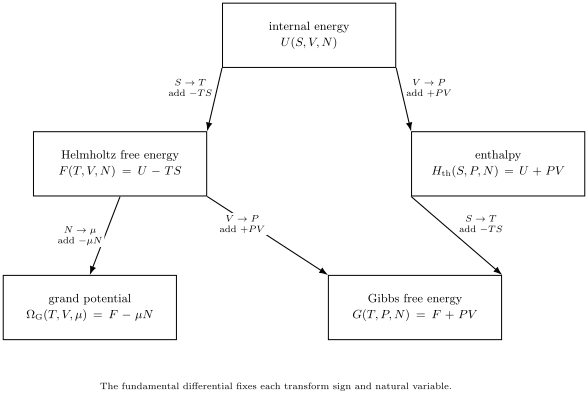
Each arrow replaces an extensive natural variable by its conjugate intensive variable. The sign of the added term follows the fundamental differential $dU=T\,dS-P\,dV+\mu\,dN$.

For stable equilibrium, it is often safer to formulate the transform variationally:

$$F(T,V,N) = \inf_S \left[ U(S,V,N)-TS \right].$$

Likewise,

$$\begin{aligned} G(T,P,N) &= \inf_V \left[ F(T,V,N)+PV \right], \\ \Omega_{\mathrm G}(T,V,\mu) &= \inf_N \left[ F(T,V,N)-\mu N \right]. \end{aligned}$$

These are Legendre–Fenchel transforms. When the relevant function is differentiable and has the required convexity, the infimum occurs at the familiar stationary condition and the construction reduces to the ordinary Legendre transform. At a first-order transition, a range of coexisting states can share the same supporting tangent, so derivatives may be discontinuous or set-valued.

The Potential Family

Internal energy

The internal energy has natural variables $S,V,N$:

$$U=U(S,V,N),$$

with

$$dU = T\,dS - P\,dV + \mu\,dN.$$

At fixed $S,V,N$, stable equilibrium minimizes $U$ against allowed internal variations. The equivalent entropy principle maximizes $S$ at fixed $U,V,N$.

Enthalpy

Enthalpy is

$$H_{\mathrm{th}} = U+PV.$$

Its differential is

$$dH_{\mathrm{th}} = T\,dS + V\,dP + \mu\,dN.$$

Its natural variables are $S,P,N$. Enthalpy is useful for mechanically open processes at fixed pressure, even though it is less often the primary potential in quantum statistical calculations.

Helmholtz free energy

The Helmholtz free energy is

$$F = U-TS.$$

Its differential is

$$dF = -S\,dT - P\,dV + \mu\,dN.$$

Its natural variables are $T,V,N$. It is the equilibrium potential of the canonical ensemble:

$$F(T,V,N) = -k_{\mathrm B}T \ln Z_N(T,V).$$

At fixed $T,V,N$, the equilibrium canonical state minimizes the Helmholtz free-energy functional.

Gibbs free energy

The Gibbs free energy is

$$G = U-TS+PV = F+PV.$$

Its differential is

$$dG = -S\,dT + V\,dP + \mu\,dN.$$

Its natural variables are $T,P,N$. At fixed temperature, pressure, and particle number, stable equilibrium minimizes $G$.

The Gibbs free energy is not generally $-k_{\mathrm B}T\ln Z_N$. That expression is the Helmholtz free energy because $Z_N$ is defined at fixed volume. A fixed-pressure ensemble requires an additional sum or integral over volumes.

Grand potential

The grand potential is

$$\Omega_{\mathrm G} = U-TS-\mu N = F-\mu N.$$

Its differential is

$$d\Omega_{\mathrm G} = -S\,dT - P\,dV - N\,d\mu.$$

Its natural variables are $T,V,\mu$. It is the equilibrium potential of the grand-canonical ensemble:

$$\Omega_{\mathrm G}(T,V,\mu) = -k_{\mathrm B}T \ln\Xi(T,V,\mu).$$

At fixed $T,V,\mu$, the equilibrium grand-canonical state minimizes the grand-potential functional.

Natural Variables and Equations of State

Once a potential is known as a function of its natural variables, its first derivatives recover the conjugate observables.

For $F(T,V,N)$,

$$\begin{aligned} S &= - \left( \frac{\partial F}{\partial T} \right)_{V,N}, \\ P &= - \left( \frac{\partial F}{\partial V} \right)_{T,N}, \\ \mu &= \left( \frac{\partial F}{\partial N} \right)_{T,V}. \end{aligned}$$

For $G(T,P,N)$,

$$\begin{aligned} S &= - \left( \frac{\partial G}{\partial T} \right)_{P,N}, \\ V &= \left( \frac{\partial G}{\partial P} \right)_{T,N}, \\ \mu &= \left( \frac{\partial G}{\partial N} \right)_{T,P}. \end{aligned}$$

For $\Omega_{\mathrm G}(T,V,\mu)$,

$$\begin{aligned} S &= - \left( \frac{\partial\Omega_{\mathrm G}}{\partial T} \right)_{V,\mu}, \\ P &= - \left( \frac{\partial\Omega_{\mathrm G}}{\partial V} \right)_{T,\mu}, \\ N &= - \left( \frac{\partial\Omega_{\mathrm G}}{\partial\mu} \right)_{T,V}. \end{aligned}$$

Every derivative must state what is held fixed. For example, differentiating with respect to $T$ at fixed $\mu$ is not the same operation as differentiating at fixed fugacity $z=e^{\beta\mu}$.

Quantum Statistical Formulas

Canonical partition function

For a fixed-$N$ Hilbert space $\mathcal H_N$,

$$Z_N(\beta,V) = \operatorname{Tr}_{\mathcal H_N} e^{-\beta\hat H_N(V)}.$$

The canonical state is

$$\rho_{N,\beta} = \frac{e^{-\beta\hat H_N}}{Z_N},$$

and

$$F = -\frac{1}{\beta} \ln Z_N.$$

For a temperature-independent Hamiltonian,

$$U = - \left( \frac{\partial\ln Z_N}{\partial\beta} \right)_{V,N}.$$

Using $F=U-TS$ gives

$$S = k_{\mathrm B} \left( \ln Z_N+\beta U \right).$$

The Canonical Ensemble page develops the state, energy fluctuations, and fixed-$N$ examples in detail.

Grand partition function

For a number-conserving Hamiltonian on Fock space,

$$\Xi(\beta,V,\mu) = \operatorname{Tr}_{\mathcal F} e^{-\beta(\hat H-\mu\hat N)}.$$

Then

$$\Omega_{\mathrm G} = -\frac{1}{\beta} \ln\Xi,$$

and

$$\begin{aligned} N &= \frac{1}{\beta} \left( \frac{\partial\ln\Xi}{\partial\mu} \right)_{\beta,V}, \\ U &= - \left( \frac{\partial\ln\Xi}{\partial\beta} \right)_{\mu,V} + \mu N. \end{aligned}$$

The $\beta$ derivative produces $\langle\hat H-\mu\hat N\rangle$, so the $\mu N$ term is required to recover the internal energy. The Grand-Canonical Ensemble page owns the Fock-space construction, fugacity, and number fluctuations.

Fixed-pressure partition function

A formal isothermal–isobaric partition function for fixed $N$ is

$$\Delta_N(\beta,P) = \frac{1}{V_0} \int_0^\infty dV\, e^{-\beta PV} Z_N(\beta,V),$$

where $V_0$ is a reference volume required to make the integral dimensionless. With this convention,

$$G_\Delta = -k_{\mathrm B}T \ln\Delta_N,$$

and

$$\left( \frac{\partial G_\Delta}{\partial P} \right)_{T,N} = \langle V\rangle.$$

Changing $V_0$ changes $G_\Delta$ by a finite additive convention. For a macroscopic system, the convention is subextensive and the saddle point yields the thermodynamic Gibbs free energy. For confined quantum systems, changing $V$ also changes the Hilbert space or boundary conditions, so the family $\hat H(V)$ must be specified.

Massieu functions

Logarithms of partition functions are dimensionless thermodynamic potentials:

$$\begin{aligned} \ln Z_N &= -\beta F, \\ \ln\Xi &= -\beta\Omega_{\mathrm G}. \end{aligned}$$

These are often called Massieu functions or Massieu–Planck potentials. They are especially convenient because derivatives with respect to dimensionless sources generate cumulants directly. Their generating role is developed on Partition Functions.

Free-Energy Variational Principles

Define the quantum relative entropy

$$D(\rho\Vert\sigma) = \operatorname{Tr} \left[ \rho \left( \ln\rho- \ln\sigma \right) \right].$$

For the canonical Gibbs state $\rho_{N,\beta}$,

$$\mathcal F_T[\rho] = \operatorname{Tr}(\rho\hat H_N) - T S(\rho)$$

satisfies

$$\mathcal F_T[\rho]-F = k_{\mathrm B}T D(\rho\Vert\rho_{N,\beta}) \geq 0.$$

Thus the Gibbs state is the unique minimizer when the relative entropy is finite and the equilibrium state has full support on the relevant space.

In the grand-canonical setting, define

$$\mathcal W_{T,\mu}[\rho] = \operatorname{Tr} \left[ \rho (\hat H-\mu\hat N) \right] - T S(\rho).$$

Then

$$\mathcal W_{T,\mu}[\rho] - \Omega_{\mathrm G} = k_{\mathrm B}T D(\rho\Vert\rho_{\beta,\mu}) \geq 0.$$

This identity is the microscopic quantum form of the thermodynamic minimum principle. Relative Entropy owns the mathematical properties of $D(\rho\Vert\sigma)$.

Pressure

Pressure is the generalized force conjugate to volume. In the canonical representation,

$$P = - \left( \frac{\partial F}{\partial V} \right)_{T,N}.$$

If the Hamiltonian depends smoothly on a geometric parameter $V$, the parameter-derivative identity gives

$$\left( \frac{\partial F}{\partial V} \right)_{T,N} = \left\langle \frac{\partial\hat H}{\partial V} \right\rangle,$$

so

$$P = - \left\langle \frac{\partial\hat H}{\partial V} \right\rangle.$$

This compact formula hides geometric choices. One must specify how the boundary, metric, couplings, and ultraviolet regulator change with $V$. In a lattice system, for example, changing the number of sites is not an infinitesimal deformation of a fixed Hilbert space.

In the grand-canonical representation,

$$P = - \left( \frac{\partial\Omega_{\mathrm G}}{\partial V} \right)_{T,\mu}.$$

For a homogeneous extensive phase in the thermodynamic limit,

$$\Omega_{\mathrm G} = -PV.$$

Surface terms, traps, interfaces, long-range interactions, and finite-size corrections can invalidate the simple identity even though the derivative definition remains meaningful.

Chemical Potential

The chemical potential is conjugate to particle number:

$$\mu = \left( \frac{\partial U}{\partial N} \right)_{S,V} = \left( \frac{\partial F}{\partial N} \right)_{T,V} = \left( \frac{\partial G}{\partial N} \right)_{T,P}.$$

In a finite quantum system, $N$ is integer-valued. Addition and removal chemical potentials are then finite differences:

$$\begin{aligned} \mu_+(N) &= F_{N+1}-F_N, \\ \mu_-(N) &= F_N-F_{N-1}. \end{aligned}$$

They can differ across a finite-size or many-body gap. A smooth derivative emerges after an interpolation or in an appropriate thermodynamic limit.

In the grand-canonical ensemble, $\mu$ is a reservoir parameter and Lagrange multiplier. It controls the probability distribution over exact number sectors; it is not generally equal to a one-particle energy. Chemical Potential owns its finite-system, fermionic, bosonic, electrochemical, and sign-convention subtleties.

Entropy from Potentials

For canonical equilibrium,

$$S = - \left( \frac{\partial F}{\partial T} \right)_{V,N} = \frac{U-F}{T}.$$

For grand-canonical equilibrium,

$$S = - \left( \frac{\partial\Omega_{\mathrm G}}{\partial T} \right)_{V,\mu} = \frac{ U-\mu N- \Omega_{\mathrm G} }{T}.$$

For a microcanonical equilibrium family, entropy is primary and determines the intensive variables through

$$\frac{1}{T} = \left( \frac{\partial S}{\partial U} \right)_{V,N}.$$

The Microcanonical Ensemble owns energy-shell definitions and finite-system entropy conventions. Entropy Overview distinguishes von Neumann entropy from purity and classical uncertainty. Entropy in Quantum Statistical Mechanics owns the systematic comparison among thermal, microcanonical, entanglement, and coarse-grained entropies.

Extensivity and Euler Relation

Suppose the internal energy is first-order homogeneous in its extensive variables:

$$U(\lambda S,\lambda V,\lambda N) = \lambda U(S,V,N).$$

Euler’s theorem then gives

$$U = TS - PV + \mu N.$$

Consequently,

$$\begin{aligned} F &= -PV+\mu N, \\ G &= \mu N, \\ \Omega_{\mathrm G} &= -PV. \end{aligned}$$

These are Euler relations for a homogeneous, one-component, extensive phase. They are not definitions valid for every finite or inhomogeneous system.

For several conserved species,

$$dU = T\,dS - P\,dV + \sum_a \mu_a\,dN_a,$$

and extensivity gives

$$U = TS-PV + \sum_a \mu_a N_a.$$

Therefore

$$G = \sum_a \mu_aN_a.$$

Gibbs–Duhem Relation

Differentiate the Euler relation:

$$\begin{aligned} dU &= T\,dS + S\,dT - P\,dV - V\,dP \\ &\quad + \mu\,dN + N\,d\mu. \end{aligned}$$

Subtracting the fundamental relation leaves

$$S\,dT - V\,dP + N\,d\mu = 0.$$

This is the Gibbs–Duhem relation. It shows that $T,P,$ and $\mu$ are not independent for a homogeneous one-component equilibrium phase.

Writing entropy and volume per particle as

$$s=\frac{S}{N}, \qquad v=\frac{V}{N},$$

gives

$$d\mu = -s\,dT + v\,dP.$$

For multiple species,

$$S\,dT - V\,dP + \sum_a N_a\,d\mu_a = 0.$$

Maxwell Relations

Mixed partial derivatives of a smooth thermodynamic potential commute. From

$$dF = -S\,dT-P\,dV+\mu\,dN,$$

one obtains

$$\left( \frac{\partial S}{\partial V} \right)_{T,N} = \left( \frac{\partial P}{\partial T} \right)_{V,N},$$ $$\left( \frac{\partial S}{\partial N} \right)_{T,V} = - \left( \frac{\partial\mu}{\partial T} \right)_{V,N},$$

and

$$\left( \frac{\partial P}{\partial N} \right)_{T,V} = - \left( \frac{\partial\mu}{\partial V} \right)_{T,N}.$$

From $G(T,P,N)$,

$$\left( \frac{\partial S}{\partial P} \right)_{T,N} = - \left( \frac{\partial V}{\partial T} \right)_{P,N}.$$

From $\Omega_{\mathrm G}(T,V,\mu)$,

$$\left( \frac{\partial S}{\partial\mu} \right)_{T,V} = \left( \frac{\partial N}{\partial T} \right)_{V,\mu},$$

and

$$\left( \frac{\partial P}{\partial\mu} \right)_{T,V} = \left( \frac{\partial N}{\partial V} \right)_{T,\mu}.$$

Maxwell relations are consistency conditions and computational tools. They are valid only where the potential is differentiable and the same variables are held fixed on both sides.

Curvature and Stability

Thermodynamic stability constrains second derivatives. At fixed $V,N$,

$$\left( \frac{\partial^2F}{\partial T^2} \right)_{V,N} = - \frac{C_{V,N}}{T} \leq 0,$$

where

$$C_{V,N} = T \left( \frac{\partial S}{\partial T} \right)_{V,N}.$$

Thus $F$ is concave in temperature for a stable canonical system.

The isothermal compressibility is

$$\kappa_T = - \frac{1}{V} \left( \frac{\partial V}{\partial P} \right)_{T,N}.$$

Mechanical stability requires $\kappa_T\geq0$, so

$$\left( \frac{\partial^2F}{\partial V^2} \right)_{T,N} = - \left( \frac{\partial P}{\partial V} \right)_{T,N} = \frac{1}{V\kappa_T} \geq 0.$$

Particle-number stability similarly requires

$$\left( \frac{\partial\mu}{\partial N} \right)_{T,V} \geq 0$$

in a stable single phase.

Grand-canonically,

$$\left( \frac{\partial^2\Omega_{\mathrm G}} {\partial\mu^2} \right)_{T,V} = - \left( \frac{\partial N}{\partial\mu} \right)_{T,V} = -\beta \operatorname{Var}(\hat N) \leq 0.$$

The final equality assumes $[\hat H,\hat N]=0$. It links thermodynamic concavity to a nonnegative quantum fluctuation. More general sources require the Kubo–Mori treatment developed in Fluctuations and Susceptibilities.

A potential can be concave in some natural variables and convex in others. Saying simply that “free energy is convex” is incomplete unless the variables are named.

Phase Coexistence

For a homogeneous one-component phase,

$$G=\mu N.$$

Two phases $a$ and $b$ coexist when their chemical potentials are equal at the same $T$ and $P$:

$$\mu_a(T,P) = \mu_b(T,P).$$

For each phase,

$$d\mu = -s\,dT + v\,dP.$$

Differentiating the coexistence condition along the coexistence curve gives the Clapeyron equation:

$$\frac{dP}{dT} = \frac{s_b-s_a}{v_b-v_a} = \frac{L}{T(v_b-v_a)},$$

where $L=T(s_b-s_a)$ is the latent heat per particle. The relation fails at points where the simple two-phase description or the required derivatives cease to apply.

At finite size, partition functions are typically analytic and the transition is rounded. Nondifferentiable thermodynamic potentials emerge only after an appropriate large-system limit. Finite-Temperature Phase Transitions develops this nonanalytic limit, the distinction between first-order and continuous transitions, and the finite-size evidence for each.

Example: A Spin in a Magnetic Field

Consider a two-level magnetic moment with

$$\hat H(B) = -mB\,\sigma_z.$$

The energies are $-mB$ and $+mB$, so

$$Z = 2\cosh(\beta mB).$$

The Helmholtz free energy is

$$F(T,B) = -k_{\mathrm B}T \ln \left[ 2\cosh(\beta mB) \right].$$

The magnetic moment conjugate to $B$ is

$$M = - \left( \frac{\partial F}{\partial B} \right)_T = m\tanh(\beta mB).$$

The internal energy is

$$U = -mB \tanh(\beta mB),$$

and the entropy is

$$S = k_{\mathrm B} \left[ \ln \left( 2\cosh x \right) - x\tanh x \right], \qquad x=\beta mB.$$

At $B=0$, both levels are equally populated and $S=k_{\mathrm B}\ln2$. At fixed nonzero $B$, the limit $T\to0^+$ selects the lower level and $S\to0$.

The isothermal susceptibility is a curvature of the free energy:

$$\chi_T = \left( \frac{\partial M}{\partial B} \right)_T = \beta m^2 \operatorname{sech}^2(\beta mB) \geq 0.$$

This is the generalized-coordinate version of the relations between compressibility, number susceptibility, and potential curvature.

Finite Systems and Exact Transforms

Thermodynamic Legendre transforms often arise as large-system limits of exact Laplace transforms.

The grand partition function is exactly

$$\Xi(\beta,\mu) = \sum_{N=0}^{\infty} \exp \left[ -\beta \left( F_N-\mu N \right) \right].$$

Therefore

$$\Omega_{\mathrm G} = -k_{\mathrm B}T \ln \sum_N e^{-\beta(F_N-\mu N)}.$$

For a macroscopic system, the logarithm is often dominated by a narrow range of $N$, giving

$$\Omega_{\mathrm G} \simeq \inf_N \left( F_N-\mu N \right)$$

up to subextensive corrections. At finite size, the log-sum-exp is smooth and need not equal the minimum.

Similarly, using a density of states $g(E)$,

$$Z(\beta) = \int dE\, g(E)e^{-\beta E}$$

becomes, when $g(E)$ has exponential thermodynamic scaling,

$$Z(\beta) \sim \int dE\, \exp \left[ \frac{S(E)}{k_{\mathrm B}} - \beta E \right].$$

The saddle point then gives

$$F(T) \simeq \inf_E \left[ E-TS(E) \right].$$

If the entropy is not concave, the canonical transform can recover only its concave envelope. This is one route to ensemble nonequivalence in systems with long-range interactions or other failures of ordinary additivity. Such statements concern thermodynamic limits; they should not be inferred from a finite analytic partition function alone. Ensemble Equivalence owns the supporting-line and large-deviation criteria.

Generalized Work Coordinates

Let the Hamiltonian depend on a control parameter $\lambda$:

$$\hat H=\hat H(\lambda).$$

For a canonical Gibbs state,

$$\left( \frac{\partial F}{\partial\lambda} \right)_T = \left\langle \frac{\partial\hat H}{\partial\lambda} \right\rangle.$$

If the generalized force is defined by

$$X_\lambda = - \frac{\partial\hat H}{\partial\lambda},$$

then

$$\langle X_\lambda\rangle = - \left( \frac{\partial F}{\partial\lambda} \right)_T.$$

Examples include magnetization conjugate to magnetic field, polarization conjugate to electric field, and stress conjugate to strain. Electromagnetic and elastic work conventions differ across subfields, so the Hamiltonian coupling should determine the sign.

Practical Workflow

For a new equilibrium problem:

1. List the exchanges. Decide whether energy, volume, particles, or another extensive quantity crosses the system boundary.
2. Identify the controls. Record which of $T,P,V,N,\mu,$ and external fields are fixed.
3. Choose the natural potential. Match the controls to $S,U,F,G,$ or $\Omega_{\mathrm G}$.
4. Specify the trace space. Use a fixed-$N$ Hilbert space for $Z_N$ and Fock space for $\Xi$.
5. Write the potential from the partition function. Keep $F=-k_{\mathrm B}T\ln Z_N$ distinct from $\Omega_{\mathrm G}=-k_{\mathrm B}T\ln\Xi$.
6. Differentiate at fixed natural variables. State every held-fixed condition.
7. Check stability. Test heat capacity, compressibility, number susceptibility, or the appropriate Hessian.
8. Check scaling. Use Euler relations such as $\Omega_{\mathrm G}=-PV$ only after verifying extensivity and homogeneity.
9. Check finite-size conventions. Replace smooth $N$ derivatives by finite differences when necessary, and retain surface terms when they matter.

Canonical Boundaries

This page owns:

• the systematic relation among $U,S,H_{\mathrm{th}},F,G,$ and $\Omega_{\mathrm G}$;
• natural variables and Legendre transforms;
• the reservoir logic selecting a potential;
• Euler, Gibbs–Duhem, Maxwell, and curvature identities;
• the distinction between exact finite-system sums and thermodynamic Legendre transforms.

Other pages own:

• quantum state construction and ensemble choice: Statistical Ensembles Overview;
• entropy maximization and the dual multiplier construction: Maximum Entropy Principle;
• fixed-$N$ Gibbs states and energy fluctuations: Canonical Ensemble;
• particle exchange and number fluctuations: Grand-Canonical Ensemble;
• static response matrices and their fluctuation representation: Fluctuations and Susceptibilities;
• trace formulas, factorization, and cumulant generation: Partition Functions;
• energy shells and microcanonical entropy conventions: Microcanonical Ensemble;
• operational heat, work, and entropy production: Energy, Heat, and Work.

Common Mistakes

Using the wrong natural variables

$F$ is natural at fixed $T,V,N$; $G$ is natural at fixed $T,P,N$; $\Omega_{\mathrm G}$ is natural at fixed $T,V,\mu$. A derivative taken while holding the wrong variables fixed computes a different response.

Calling every free energy the Gibbs free energy

$-k_{\mathrm B}T\ln Z_N$ is the Helmholtz free energy. Gibbs free energy requires fixed pressure and includes $PV$.

Forgetting the pressure sign

The fundamental relation contains $-P\,dV$, so $P=-\partial F/\partial V$. Enthalpy and Gibbs free energy contain $+PV$.

Confusing the Hamiltonian with enthalpy

Both are often denoted $H$. Here $\hat H$ is the quantum Hamiltonian and $H_{\mathrm{th}}=U+PV$ is enthalpy.

Applying Ω = −PV to every system

The identity requires a homogeneous extensive phase in the thermodynamic limit. Traps, surfaces, interfaces, and long-range interactions can add corrections.

Treating finite particle number as continuous

For finite $N$, chemical potentials are naturally addition and removal differences. A smooth derivative is a macroscopic approximation or interpolation.

Replacing a finite log-sum-exp by a minimum

The grand potential is exactly a logarithm of a sum over sectors. The Legendre minimum is a dominant-sector approximation in an appropriate large-system limit.

Assuming all curvatures have the same sign

$F$ is concave in $T$ but convex in stable mechanical extensive variables such as $V$. Curvature statements must name the variable.

Imposing equilibrium monotonicity on a driven process

Minimum principles compare equilibrium candidates under fixed reservoir controls. Nonequilibrium work protocols require additional definitions and inequalities.

Exercises

Reconstruct the potential differentials

Starting from

$$dU = T\,dS-P\,dV+\mu\,dN,$$

derive the differentials of $H_{\mathrm{th}}$, $F$, $G$, and $\Omega_{\mathrm G}$. Identify the natural variables of each potential.

Solution

For enthalpy,

$$H_{\mathrm{th}} = U+PV,$$

so

$$\begin{aligned} dH_{\mathrm{th}} &= dU+P\,dV+V\,dP \\ &= T\,dS+V\,dP+\mu\,dN. \end{aligned}$$

Its natural variables are $S,P,N$.

For Helmholtz free energy,

$$F=U-TS,$$

and therefore

$$dF = -S\,dT-P\,dV+\mu\,dN.$$

Its natural variables are $T,V,N$.

For Gibbs free energy,

$$G=U-TS+PV,$$

which gives

$$dG = -S\,dT+V\,dP+\mu\,dN.$$

Its natural variables are $T,P,N$.

Finally,

$$\Omega_{\mathrm G} = U-TS-\mu N,$$

so

$$d\Omega_{\mathrm G} = -S\,dT-P\,dV-N\,d\mu.$$

Its natural variables are $T,V,\mu$.

Prove the canonical variational identity

Let

$$\rho_\beta = \frac{e^{-\beta\hat H}}{Z}.$$

Show that

$$\operatorname{Tr}(\rho\hat H) - TS(\rho) - F = k_{\mathrm B}T D(\rho\Vert\rho_\beta).$$

Solution

The Gibbs state satisfies

$$\ln\rho_\beta = -\beta\hat H- \ln Z.$$

Hence

$$\begin{aligned} D(\rho\Vert\rho_\beta) &= \operatorname{Tr}(\rho\ln\rho) - \operatorname{Tr}(\rho\ln\rho_\beta) \\ &= \operatorname{Tr}(\rho\ln\rho) + \beta\operatorname{Tr}(\rho\hat H) + \ln Z. \end{aligned}$$

Multiply by $k_{\mathrm B}T=1/\beta$ and use

$$S(\rho) = -k_{\mathrm B} \operatorname{Tr}(\rho\ln\rho)$$

and

$$F = -k_{\mathrm B}T\ln Z.$$

This gives

$$k_{\mathrm B}T D(\rho\Vert\rho_\beta) = \operatorname{Tr}(\rho\hat H) - TS(\rho) - F.$$

Since relative entropy is nonnegative, $\rho_\beta$ minimizes the free-energy functional.

Magnetic two-level system

For

$$\hat H=-mB\sigma_z,$$

derive $F$, $M$, and $\chi_T$. Check the limits $B\to0$ and $T\to0^+$.

Solution

The two energies are $\mp mB$, so

$$Z = e^{\beta mB} + e^{-\beta mB} = 2\cosh(\beta mB).$$

Therefore

$$F = -k_{\mathrm B}T \ln \left[ 2\cosh(\beta mB) \right].$$

The conjugate magnetic moment is

$$M = - \left( \frac{\partial F}{\partial B} \right)_T = m\tanh(\beta mB).$$

Differentiating again,

$$\chi_T = \left( \frac{\partial M}{\partial B} \right)_T = \beta m^2 \operatorname{sech}^2(\beta mB).$$

For weak field,

$$M \simeq \beta m^2B,$$

which is the Curie-law response of one independent moment. At fixed nonzero $B$ and $T\to0^+$,

$$M \to m\,\operatorname{sgn}(B),$$

while $\chi_T\to0$ away from $B=0$ because the ground state is saturated.

Maxwell relation and thermal expansion

Use $G(T,P,N)$ to prove

$$\left( \frac{\partial S}{\partial P} \right)_{T,N} = - \left( \frac{\partial V}{\partial T} \right)_{P,N}.$$

Express the right-hand side using the thermal expansion coefficient

$$\alpha_P = \frac{1}{V} \left( \frac{\partial V}{\partial T} \right)_{P,N}.$$

Solution

From

$$dG = -S\,dT+V\,dP+\mu\,dN,$$

we have

$$S = - \left( \frac{\partial G}{\partial T} \right)_{P,N}, \qquad V = \left( \frac{\partial G}{\partial P} \right)_{T,N}.$$

Commuting the mixed derivatives gives

$$\begin{aligned} \left( \frac{\partial S}{\partial P} \right)_{T,N} &= - \frac{\partial^2G} {\partial P\,\partial T} \\ &= - \left( \frac{\partial V}{\partial T} \right)_{P,N}. \end{aligned}$$

Therefore

$$\left( \frac{\partial S}{\partial P} \right)_{T,N} = -V\alpha_P.$$

A material that expands on heating at fixed pressure has entropy that decreases with increasing pressure at fixed temperature.

Gibbs–Duhem and Clapeyron

Assume $U(S,V,N)$ is first-order homogeneous. Derive the Gibbs–Duhem relation and then derive the Clapeyron equation for coexistence between phases $a$ and $b$.

Solution

Euler’s theorem gives

$$U = TS-PV+\mu N.$$

Differentiating,

$$\begin{aligned} dU &= T\,dS-P\,dV+\mu\,dN \\ &\quad + S\,dT-V\,dP+N\,d\mu. \end{aligned}$$

Comparison with the fundamental relation leaves

$$S\,dT-V\,dP+N\,d\mu = 0.$$

Dividing by $N$ gives

$$d\mu = -s\,dT+v\,dP.$$

Along coexistence,

$$\mu_a(T,P) = \mu_b(T,P).$$

Their differentials must also agree:

$$-s_a\,dT+v_a\,dP = -s_b\,dT+v_b\,dP.$$

Rearranging gives

$$\frac{dP}{dT} = \frac{s_b-s_a}{v_b-v_a}.$$

Since the latent heat per particle is

$$L = T(s_b-s_a),$$

the result is

$$\frac{dP}{dT} = \frac{L}{T(v_b-v_a)}.$$

Finite-sector transform

Suppose only the sectors $N=0$ and $N=1$ are available, with

$$F_0=0, \qquad F_1=\epsilon.$$

Compute $\Xi$, $\Omega_{\mathrm G}$, and $\langle N\rangle$. Compare the exact grand potential with the Legendre minimum of $F_N-\mu N$.

Solution

The sector sum is

$$\Xi = 1 + e^{-\beta(\epsilon-\mu)}.$$

Therefore

$$\Omega_{\mathrm G} = -k_{\mathrm B}T \ln \left[ 1+e^{-\beta(\epsilon-\mu)} \right].$$

The mean occupation is

$$\langle N\rangle = \frac{1}{\beta} \frac{\partial\ln\Xi}{\partial\mu} = \frac{1}{e^{\beta(\epsilon-\mu)}+1}.$$

The two values of $F_N-\mu N$ are

$$0 \qquad\text{and}\qquad \epsilon-\mu.$$

Their minimum is

$$\min \left( 0, \epsilon-\mu \right).$$

At finite temperature, the exact $\Omega_{\mathrm G}$ is a smooth log-sum-exp and lies below or equal to this minimum. In the limit $T\to0^+$,

$$\Omega_{\mathrm G} \to \min \left( 0, \epsilon-\mu \right),$$

while $\langle N\rangle$ approaches a step function, with a degeneracy at $\mu=\epsilon$.

Cross-Links

• Statistical Ensembles Overview
• Microcanonical Ensemble
• Thermal Density Operators
• Canonical Ensemble
• Grand-Canonical Ensemble
• Partition Functions
• Entropy in Quantum Statistical Mechanics
• Maximum Entropy Principle
• Chemical Potential
• Ensemble Equivalence
• Thermodynamic Limit
• Ensemble Formula Sheet
• Relative Entropy
• Entropy Overview
• Energy, Heat, and Work

References

• H. B. Callen, Thermodynamics and an Introduction to Thermostatistics, 2nd ed., Wiley (1985), chapters 1–8.
• R. K. Pathria and P. D. Beale, Statistical Mechanics, 4th ed., Elsevier (2021), chapters 2–5.
• M. Kardar, Statistical Physics of Particles, Cambridge University Press (2007), chapters 1, 4, and 6.
• L. D. Landau and E. M. Lifshitz, Statistical Physics, Part 1, 3rd ed., Butterworth–Heinemann (1980), sections 13–24 and 31–36.
• T. L. Hill, Thermodynamics of Small Systems, Dover (1994), parts I and II.
• H. Touchette, “The Large Deviation Approach to Statistical Mechanics”, Physics Reports 478, 1–69 (2009).
• R. Balian, From Microphysics to Macrophysics, Volume I, Springer (1991), chapters 4–7.