Ensemble Equivalence

Ensemble equivalence is an asymptotic statement that differently constrained equilibrium ensembles can give the same selected macroscopic or local predictions after their thermodynamic parameters are matched. It is not an identity between finite-system density operators.

The microcanonical ensemble fixes an energy shell. The canonical ensemble fixes temperature and allows energy to fluctuate. The canonical fixed-$N$ ensemble and the grand-canonical ensemble similarly differ over whether particle number is exact or fluctuating. For ordinary additive matter, these distinctions often become invisible to local bulk observables as the system grows. They remain visible to exact constraints, global fluctuations, rare events, and finite-size corrections. Fluctuations and Susceptibilities organizes those global differences and their relation to response.

A trustworthy equivalence claim must answer four questions:

1. Which ensembles are being compared?
2. How are their parameters matched?
3. Which observables or thermodynamic functions are compared?
4. Which sequence of systems and limit justifies the comparison?

The Short Answer

Microcanonical and canonical predictions commonly agree when:

• a regular thermodynamic limit exists;
• interactions are short ranged enough for boundary interactions to be subextensive;
• the system is additive and thermodynamically stable;
• the matched energy density lies in a concave region of the entropy;
• the equilibrium macrostate is selected consistently;
• the observable is local or grows slowly compared with the whole system;
• the microcanonical window contains many levels while remaining narrow on the macroscopic scale.

Canonical and grand-canonical predictions commonly agree under analogous conditions when the number density concentrates, the compressibility is regular, and the fixed-number and fluctuating-number ensembles are matched by

$$\overline N_{\beta,\mu} = N.$$

Important qualifications include:

• finite systems;
• observables sensitive to exact global conservation;
• first-order coexistence and nonunique phases;
• critical points with divergent correlation length;
• nonadditive long-range interactions;
• nonconcave entropy;
• incompatible symmetry sectors or boundary conditions;
• additional conserved quantities retained by the preparation.

None of these words is a substitute for checking the actual limit.

Finite-Volume Definitions

Let a finite region $\Lambda_V$ have volume or site count $V$ and Hamiltonian $H_V$. A canonical state is

$$\rho_{\beta,V}^{\mathrm{can}} = \frac{ e^{-\beta H_V} }{ Z_V(\beta) }, \qquad Z_V(\beta) = \operatorname{Tr} e^{-\beta H_V}.$$

For an energy window

$$[E,E+\Delta],$$

let $\Pi_{V,E,\Delta}$ be the corresponding spectral projector. The microcanonical state is

$$\rho_{V,E,\Delta}^{\mathrm{mc}} = \frac{ \Pi_{V,E,\Delta} }{ \Omega_V(E,\Delta) },$$

where

$$\Omega_V(E,\Delta) = \operatorname{Tr} \Pi_{V,E,\Delta}.$$

The natural first matching condition is

$$E \simeq \operatorname{Tr} \left( \rho_{\beta,V}^{\mathrm{can}}H_V \right).$$

At finite $V$, the states are normally different:

• the microcanonical state has support only in its chosen shell;
• the canonical state has weights across many energies;
• microcanonical energy variance is controlled by $\Delta$;
• canonical energy variance is set by heat capacity;
• exact finite-size expectation values need not agree.

The question is not whether these distinctions literally disappear at a finite size. It is whether a declared difference tends to zero along a declared thermodynamic sequence.

Choosing the Microcanonical Window

The shell width must resolve two competing requirements. It should be:

• much larger than the many-body level spacing, so the shell contains enough states for stable statistics;
• subextensive, so its energy-density width vanishes as $V\to\infty$.

A common asymptotic condition is

$$\Delta_V=o(V),$$

combined with

$$\Omega_V(E_V,\Delta_V)\to\infty.$$

Particular theorems impose stronger lower and upper bounds. A window narrower than a sparse spectrum can be empty or dominated by accidental degeneracy. A window of order $V$ does not define a sharp energy density.

The window convention also affects finite-size entropy and fluctuation estimates. Equivalence claims should therefore state $\Delta_V$ or at least its scaling.

Several Levels of Equivalence

The word equivalence is used for distinct claims. They should not be merged.

Thermodynamic equivalence

Thermodynamic potentials obtained from different ensembles are related by the expected Legendre–Fenchel transforms, and equations of state agree after matching intensive and extensive variables.

This is a statement about limiting functions such as entropy density, free-energy density, pressure, and their regular derivatives.

Equilibrium-macrostate equivalence

The ensembles select the same set of equilibrium values for macroscopic observables such as density, magnetization, or an order parameter.

Two ensembles can have related thermodynamic potentials while differing in which phase mixture or macrostate is selected at a nondifferentiable point.

Local-state equivalence

Reduced density operators on a fixed or sufficiently slowly growing region become indistinguishable:

$$\frac12 \left\| \rho_{B,V}^{\mathrm{mc}} - \rho_{B,V}^{\mathrm{can}} \right\|_1 \longrightarrow 0.$$

Here

$$\rho_{B,V}^{\mathrm{mc}} = \operatorname{Tr}_{\overline B} \rho_{V,E,\Delta}^{\mathrm{mc}}, \qquad \rho_{B,V}^{\mathrm{can}} = \operatorname{Tr}_{\overline B} \rho_{\beta,V}^{\mathrm{can}}.$$

For any observable $A_B$ supported in $B$,

$$\left| \langle A_B\rangle_{\mathrm{mc}} - \langle A_B\rangle_{\mathrm{can}} \right| \leq \left\|A_B\right\|_\infty \left\| \rho_{B,V}^{\mathrm{mc}} - \rho_{B,V}^{\mathrm{can}} \right\|_1.$$

This is the most directly quantum-mechanical form of local ensemble equivalence.

Measure or specific-relative-entropy equivalence

A useful global but weak criterion is that relative entropy per volume vanishes:

$$\frac{1}{V} D \left( \rho_{V}^{\mathrm{mc}} \middle\| \rho_{V}^{\mathrm{can}} \right) \longrightarrow 0.$$

Subextensive relative entropy does not require the global trace distance to vanish. It is compatible with different exact constraints and different fluctuations of extensive quantities.

Fluctuation equivalence

Agreement of mean densities does not imply agreement of fluctuation distributions. One may separately ask whether variances, central-limit scaling, higher cumulants, or large-deviation rate functions agree.

The strongest version is rarely what a textbook means by “equivalence of ensembles.”

Thermodynamic Scaling

Define energy density

$$e = \frac EV.$$

Suppose the number of states in a suitable shell has exponential scaling

$$\Omega_V(Ve,\Delta_V) \asymp \exp \left[ V\sigma(e) \right],$$

where

$$\sigma(e) = \frac{s(e)}{k_{\mathrm B}}$$

is the dimensionless entropy density. The symbol $\asymp$ means equality at leading exponential order:

$$\lim_{V\to\infty} \frac{1}{V} \ln \Omega_V(Ve,\Delta_V) = \sigma(e).$$

Define the dimensionless canonical potential density

$$\varphi(\beta) \equiv - \lim_{V\to\infty} \frac{1}{V} \ln Z_V(\beta).$$

It is related to the free-energy density $f(\beta)$ by

$$\varphi(\beta) = \beta f(\beta).$$

Exact Laplace Sum and Saddle Point

Group the canonical partition function by energy shells. At leading exponential order,

$$\begin{aligned} Z_V(\beta) &\sim \int de\, \exp \left\{ V \left[ \sigma(e)-\beta e \right] \right\}. \end{aligned}$$

Laplace’s method gives

$$\varphi(\beta) = \inf_e \left[ \beta e-\sigma(e) \right].$$

The finite-system partition function remains an exact sum or trace. The variational expression is the thermodynamic leading order, not a replacement for the finite log-sum-exp.

If $\sigma$ is differentiable and the minimizer is interior, stationarity gives

$$\beta = \sigma'(e_\beta).$$

Since

$$\beta = \frac{1}{k_{\mathrm B}T},$$

this is the entropy-representation definition of temperature.

Supporting Lines and Concavity

A line of slope $\beta$ supports $\sigma(e)$ at $e_*$ when

$$\sigma(e) \leq \sigma(e_*) + \beta(e-e_*)$$

for every allowed $e$.

Equivalently, $e_*$ minimizes

$$\beta e-\sigma(e).$$

The canonical ensemble can realize $e_*$ as a typical equilibrium energy density only if such a supporting line exists.

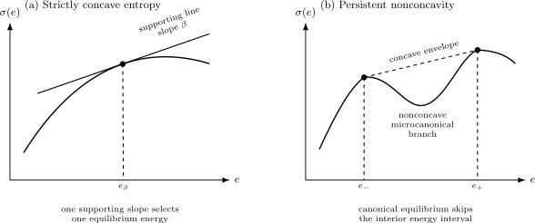
Left: strict concavity gives a unique matched energy $e_\beta$ for the supporting slope $\beta$. Right: a persistent nonconcave region lies below the concave envelope; canonical equilibrium at the coexistence slope selects the contact energies $e_-$ and $e_+$ rather than the intervening microcanonical branch.

Three cases should be distinguished.

Strictly concave entropy

If $\sigma(e)$ is strictly concave and differentiable, each interior energy has a unique supporting slope

$$\beta=\sigma'(e),$$

and each regular $\beta$ selects a unique $e_\beta$. This is the cleanest thermodynamic equivalence regime.

Affine entropy segment

If $\sigma(e)$ is linear on an interval, one slope supports every energy in that interval. The canonical potential is nondifferentiable, and the same temperature can coexist with multiple energy densities.

This is partial rather than one-to-one equivalence. It is the thermodynamic geometry behind first-order coexistence in an additive system.

Nonconcave entropy

If

$$\sigma(e) < \sigma^{**}(e),$$

where $\sigma^{**}$ is the smallest upper semicontinuous concave envelope, then no supporting line touches $\sigma$ at that energy. The canonical ensemble skips that branch.

The inverse transform gives

$$\sigma^{**}(e) = \inf_\beta \left[ \beta e-\varphi(\beta) \right].$$

Canonical thermodynamics reconstructs $\sigma^{**}$, not the hidden nonconcave part of $\sigma$. A persistent difference

$$\sigma^{**}(e)-\sigma(e)>0$$

is a thermodynamic signature of microcanonical–canonical nonequivalence.

Large-Deviation Preview

The canonical probability of observing energy density near $e$ has the leading form

$$P_{\beta,V}(e) \asymp e^{-V I_\beta(e)}.$$

The rate function is

$$I_\beta(e) = \beta e - \sigma(e) - \varphi(\beta).$$

Because $\varphi$ is the infimum of $\beta e-\sigma(e)$,

$$I_\beta(e)\geq0.$$

Canonical equilibrium energies are exactly the global minimizers:

$$I_\beta(e)=0.$$

If there is one nondegenerate minimizer $e_\beta$, the distribution concentrates there. For every fixed $\delta>0$,

$$P_{\beta,V} \left( \left|e-e_\beta\right|>\delta \right) \sim e^{-V c_\delta}$$

with a positive rate $c_\delta$ under the usual regularity assumptions.

Large deviations do more than say that relative fluctuations vanish. They identify exponentially suppressed macroscopic energies and expose coexistence when the rate function has several minima.

Gaussian Fluctuations Near One Minimum

Suppose $I_\beta$ is twice differentiable at a unique minimum. Then

$$I_\beta(e) \simeq \frac12 I_\beta''(e_\beta) \left( e-e_\beta \right)^2.$$

The width of the energy-density distribution is then

$$\Delta e \sim V^{-1/2}.$$

Equivalently,

$$\operatorname{Var}_{\mathrm{can}}(H_V) = k_{\mathrm B}T^2 C_V.$$

If

$$C_V\sim V, \qquad \langle H_V\rangle\sim V,$$

then

$$\frac{ \sqrt{\operatorname{Var}(H_V)} }{ \left|\langle H_V\rangle\right| } \sim V^{-1/2}.$$

This concentration explains why an exact microcanonical energy and a fluctuating canonical energy can produce the same local bulk values.

The estimate requires qualification when the mean energy crosses zero, the heat capacity has anomalous finite-size scaling, the system is at coexistence, or the correlation length becomes comparable with the system size.

Why Short-Range Additivity Helps

Split a large system into macroscopic regions $A$ and $B$. For a sufficiently short-range interaction,

$$H_{A\cup B} = H_A+H_B+H_{\partial},$$

where the interaction across the boundary satisfies

$$\left\|H_{\partial}\right\| = o(V)$$

for a regular thermodynamic sequence.

The bulk energy is therefore additive at leading order. Combining states of the two regions yields the entropy inequality

$$\sigma \left( \lambda e_A+(1-\lambda)e_B \right) \geq \lambda\sigma(e_A) + (1-\lambda)\sigma(e_B)$$

in the thermodynamic limit, subject to the model’s precise assumptions. This is concavity.

Physically, if two energy densities coexist, an additive system can place one phase in part of the volume and the other phase in the remainder. The interface costs less than the bulk:

$$F_{\mathrm{interface}} = o(V).$$

This phase-separation mechanism convexifies the thermodynamic description.

Short range is not a complete theorem by itself. Stability, boundary conditions, lattice geometry, conserved sectors, existence of the limit, and regularity of the state all matter.

Local Equivalence in Quantum Lattices

For a quantum lattice Hamiltonian with short-range interactions, a canonical Gibbs state away from criticality often has a finite correlation length. A small region then couples to the rest primarily through a boundary while the complement acts as a large energy reservoir.

Rigorous finite-size results make versions of this intuition precise. Under stated locality, correlation, temperature, window, and lattice assumptions, the reduced canonical and microcanonical states approach one another on regions whose size is fixed or grows subextensively.

The exact allowed growth of the region depends on the theorem. It should not be replaced by the vague claim that “any subsystem smaller than the whole system” is thermal.

Local equivalence also does not imply that a typical pure energy eigenstate is thermal. That stronger dynamical or eigenstate-level statement belongs to typicality and the eigenstate thermalization hypothesis.

Exact Example: Independent Two-Level Sites

Consider $L$ independent two-level sites:

$$H_L = \Delta \sum_{i=1}^{L} n_i, \qquad n_i\in\{0,1\}.$$

Canonical ensemble

Each site is excited independently with probability

$$p_\beta = \frac{ e^{-\beta\Delta} }{ 1+e^{-\beta\Delta} } = \frac{1}{ e^{\beta\Delta}+1 }.$$

The total excitation number $K$ is binomial:

$$P_{\mathrm{can}}(K) = \binom{L}{K} p_\beta^K \left( 1-p_\beta \right)^{L-K}.$$

Its variance is

$$\operatorname{Var}_{\mathrm{can}}(K) = L p_\beta \left( 1-p_\beta \right).$$

Microcanonical ensemble

Fix exactly $K$ excited sites. Every bit string with that total is assigned equal weight:

$$\Omega_L(K) = \binom{L}{K}.$$

Choose a subsystem containing $r$ sites. The number $J$ of excitations in that subsystem has a hypergeometric distribution:

$$P_{\mathrm{mc}}(J=j) = \frac{ \binom{K}{j} \binom{L-K}{r-j} }{ \binom{L}{r} }.$$

In the canonical ensemble,

$$P_{\mathrm{can}}(J=j) = \binom{r}{j} p_\beta^j \left( 1-p_\beta \right)^{r-j}.$$

If

$$\frac KL \longrightarrow p_\beta$$

while $r$ remains fixed, sampling without replacement becomes sampling with replacement:

$$P_{\mathrm{mc}}(J=j) \longrightarrow P_{\mathrm{can}}(J=j).$$

Every fixed local block becomes equivalent.

Globally, however,

$$\operatorname{Var}_{\mathrm{mc}}(K)=0$$

while

$$\operatorname{Var}_{\mathrm{can}}(K) = L p_\beta(1-p_\beta).$$

The absolute variance difference grows with $L$, even though the canonical relative fluctuation of $K/L$ vanishes. This example captures the central distinction between local equivalence and global equality.

Correlations Induced by an Exact Constraint

In the fixed-$K$ ensemble,

$$\langle n_i\rangle_{\mathrm{mc}} = \frac KL.$$

For distinct sites $i\neq j$,

$$\langle n_i n_j\rangle_{\mathrm{mc}} = \frac{ K(K-1) }{ L(L-1) }.$$

Therefore

$$\operatorname{Cov}_{\mathrm{mc}}(n_i,n_j) = - \frac{ p_L(1-p_L) }{ L-1 }, \qquad p_L=\frac KL.$$

The exact global constraint creates weak anticorrelations of order $1/L$. Any fixed pair becomes independent in the limit, but summing $O(L^2)$ such correlations enforces zero variance of the total.

Small local errors can therefore combine into an order-$L$ difference for a global observable.

Canonical and Grand-Canonical Equivalence

Let $F_V(N)$ be the canonical free energy in the exact $N$ sector. The grand-canonical number probability is

$$P_{\beta,\mu,V}(N) = \frac{ e^{-\beta[F_V(N)-\mu N]} }{ \Xi_V }.$$

If

$$F_V(N) \simeq V f(n), \qquad n=\frac NV,$$

then

$$P_{\beta,\mu,V}(n) \asymp e^{-V J_{\beta,\mu}(n)}$$

for a number-density rate function $J_{\beta,\mu}$.

A unique stable minimum $n_{\beta,\mu}$ gives concentration:

$$\frac{ \sqrt{\operatorname{Var}(N)} }{ \overline N } \sim V^{-1/2}$$

when the number susceptibility is extensive and the mean density is nonzero.

The response identity

$$\left( \frac{\partial\overline N}{\partial\mu} \right)_{T,V} = \beta\operatorname{Var}(N)$$

connects regular compressibility with regular number concentration.

Local fixed-density and grand-canonical predictions can then agree after choosing $\mu$ so that

$$\frac{ \overline N_{\beta,\mu} }{ V } \longrightarrow n.$$

Exact total-number fluctuations remain different. At a density-driven first-order transition, the grand-canonical distribution can be bimodal and the matching may be nonunique.

First-Order Coexistence

Phase coexistence is a qualification, not an automatic proof of nonequivalence.

For an additive short-range system, an intermediate microcanonical energy can be realized by spatial phase separation. In the thermodynamic limit, the entropy can develop an affine segment rather than a persistent nonconcave region.

At the coexistence inverse temperature $\beta_c$:

• the canonical energy distribution can have two macroscopic peaks;
• the mean canonical energy can lie between the peak energies;
• a microcanonical state at an intermediate energy can contain an interface and a definite phase fraction;
• boundary conditions can favor one pure phase or a mixture;
• the canonical energy variance need not have ordinary $O(V)$ Gaussian scaling.

Thermodynamic potentials may still be Legendre–Fenchel equivalent, while macrostate mixtures, interfaces, and finite-size distributions differ.

Matching only the mean energy is therefore insufficient at coexistence. One must also specify boundary conditions, phase selection, observables, and the order of limits.

Finite-Size Convex Intruders

A finite short-range system may show a nonconcave-looking microcanonical entropy because an interface costs free energy. The correction often scales like an area rather than a volume.

If the interface cost is subextensive,

$$\frac{ F_{\mathrm{interface}} }{ V } \longrightarrow 0,$$

the apparent convex intruder can disappear in the entropy density. It should not be mistaken for persistent thermodynamic nonequivalence.

Finite clusters, nuclei, droplets, and trapped gases can nevertheless display physically important finite-size effects. Calling them “nonequivalent” is acceptable only when the finite-system criterion being used is stated.

Critical Points

At a continuous critical point, the correlation length can grow to the system size. Then:

• proofs requiring exponential clustering no longer apply directly;
• central-limit estimates can acquire anomalous exponents;
• finite-size corrections decay slowly;
• susceptibilities and heat capacities may scale superextensively over finite sequences;
• a local region may need to remain smaller than additional critical scales.

Failure of a sufficient theorem is not proof of nonequivalence. Many additive short-range systems remain thermodynamically equivalent at criticality, but convergence and the appropriate scaling theory are more delicate.

Long-Range and Nonadditive Interactions

Suppose the interaction between two macroscopic pieces remains of bulk order:

$$H_{A\cup B} - H_A - H_B = O(V).$$

The system is nonadditive. Spatial phase separation can no longer convexify the entropy at subextensive cost.

For pair potentials behaving asymptotically as

$$v(r) \sim \frac{1}{r^\alpha}$$

in $d$ spatial dimensions, the regime $\alpha\leq d$ is a standard source of strong long-range behavior unless screening, neutrality, geometry, or another mechanism changes the effective thermodynamics.

Rescaling the interaction to make total energy extensive does not necessarily restore additivity. Extensivity and additivity are different properties.

A nonadditive thermodynamic limit can retain

$$\sigma''(e)>0$$

on an interval. Since

$$\sigma'(e) = \frac{1}{k_{\mathrm B}T},$$

the microcanonical heat-capacity density obeys

$$c_V = - \frac{1}{ k_{\mathrm B}T^2\sigma''(e) }.$$

Thus $\sigma''(e)>0$ gives

$$c_V<0$$

microcanonically.

The canonical ensemble cannot realize a stable negative heat capacity because

$$C_V^{\mathrm{can}} = \frac{ \operatorname{Var}_{\mathrm{can}}(H) }{ k_{\mathrm B}T^2 } \geq 0.$$

The canonical distribution instead jumps between concave-envelope contact energies. This is genuine ensemble nonequivalence.

Long range permits nonequivalence; it does not guarantee it. Each model still requires analysis of stability, scaling, accessible macrostates, and entropy geometry.

Symmetry Breaking and Boundary Conditions

At finite volume with exact symmetry and no source, a Gibbs state can be a symmetric mixture even where infinite-volume pure phases break the symmetry.

To compare ensembles meaningfully, use compatible:

• boundary conditions;
• symmetry sectors;
• external sources;
• orders of $V\to\infty$ and source removal;
• phase-selection prescriptions.

Two sequences can have identical bulk free-energy density but different limiting local states because they select different pure phases. That is phase nonuniqueness, not necessarily failure of thermodynamic Legendre equivalence.

Constraints, Fragmentation, and Integrability

An ensemble averages only over the state space included in its definition. Comparing a microcanonical shell in one symmetry sector with a canonical state that mixes several sectors is not a clean test of equivalence.

If the Hilbert space fragments into dynamically disconnected components, a preparation may retain more information than energy alone. Likewise, an integrable model has many conserved quantities that can constrain post-quench relaxation.

These facts should be separated:

• equilibrium canonical and microcanonical ensembles can still be compared within a declared sector;
• a real isolated preparation may fail to approach either ordinary ensemble because extra charges remain fixed;
• a generalized Gibbs ensemble addresses those additional constraints;
• thermalization and ensemble equivalence are logically distinct.

Integrability is therefore not a universal proof that canonical and microcanonical thermodynamics are nonequivalent.

Nonequilibrium Overview owns the separate dynamical test: whether the diagonal ensemble for a prepared state is locally approximated by an ordinary or generalized equilibrium ensemble.

Negative Temperatures

A bounded spectrum can support

$$\beta<0.$$

Negative temperature does not by itself break ensemble equivalence. The same supporting-line and concavity analysis applies, now with a negative slope.

Trouble arises when entropy geometry, inaccessible sectors, nonadditivity, or limiting procedures violate the required conditions. The sign of $\beta$ alone is not the criterion.

Rare Events and Global Observables

Suppose two ensembles agree on every observable supported in a fixed region. They can still disagree on:

• total energy variance;
• total particle-number variance;
• the probability of a macroscopic fluctuation;
• full counting statistics;
• the largest cluster or global order parameter;
• topological or sector projectors spanning the system;
• interface location and phase fraction.

Large-deviation rate functions retain information beyond local expectation values. Two distributions may concentrate at the same mean while assigning exponentially different probabilities to atypical values.

Always match the strength of the equivalence claim to the observable class.

Equivalence Is Not Typicality

The microcanonical density operator is a mixed state over a shell. Canonical–microcanonical equivalence compares ensemble predictions.

Canonical typicality asks whether most pure states sampled from a constrained high-dimensional subspace have nearly canonical reduced states. Eigenstate thermalization asks whether individual energy eigenstates reproduce thermal local observables. Dynamical thermalization asks whether a prepared state approaches those predictions in time.

These ideas reinforce one another in many chaotic systems, but none follows solely from ensemble equivalence.

Equivalence Is Not a Reservoir Derivation

Deriving a canonical state for a small subsystem of a larger microcanonical whole and proving equivalence between two ensembles for the same large system are related but distinct arguments.

The subsystem derivation typically assumes:

• weak or boundary-scale coupling;
• a much larger environment;
• a smooth environment entropy;
• a narrow total-energy shell.

Ensemble equivalence instead compares limiting descriptions after macroscopic parameters are matched. One argument should not be cited as a complete proof of the other without checking assumptions.

Practical Comparison Workflow

To test an ensemble-equivalence claim:

1. Specify the finite systems. Give $H_V$, geometry, boundary conditions, and interaction scaling.
2. State the ensembles. Include trace domains, exact sectors, and shell convention.
3. Choose the matching rule. Match energy density, particle density, or conjugate derivatives.
4. Name the observable class. Local operators, thermodynamic densities, global fluctuations, or rare events.
5. Check additivity and stability. Determine whether cross-boundary interactions are subextensive.
6. Inspect entropy concavity. Look for supporting lines, affine segments, or persistent nonconcavity.
7. Check concentration. Estimate variance or a large-deviation rate function.
8. Track correlation length. Criticality can invalidate simple finite-size bounds.
9. Handle phase selection. Align boundary conditions, sources, and order of limits.
10. Separate dynamics. Do not infer thermalization or ETH from an equilibrium comparison.

Canonical Boundaries

This page owns:

• the levels at which ensembles can be equivalent;
• parameter matching and observable dependence;
• the entropy-concavity and supporting-line criterion;
• the large-deviation explanation of concentration;
• local quantum-state equivalence;
• finite-size, coexistence, critical, constrained, and long-range qualifications.

Other pages own:

• choosing among the standard ensembles: Statistical Ensembles Overview;
• microcanonical shell and entropy conventions: Microcanonical Ensemble;
• fixed-temperature Gibbs thermodynamics: Canonical Ensemble;
• fluctuating particle number and Fock-space traces: Grand-Canonical Ensemble;
• definitions and order of large-system limits: Thermodynamic Limit;
• Legendre transforms and potential curvature: Thermodynamic Potentials;
• static fluctuation scaling, susceptibilities, and critical enhancement: Fluctuations and Susceptibilities;
• finite-size-scaling algorithms and data-collapse diagnostics: computational and phase-transition pages;
• dynamical equilibration and ETH: Nonequilibrium Many-Body Dynamics.

Common Mistakes

• Saying that all ensembles are identical in the thermodynamic limit.
• Omitting the observable class from an equivalence claim.
• Comparing finite systems and calling small numerical differences a theorem.
• Matching temperature and energy without checking whether the equation of state is one-to-one.
• Using a microcanonical shell narrower than the many-body level spacing.
• Using an extensive shell width that does not select one energy density.
• Treating vanishing relative energy fluctuations as equality of global fluctuation distributions.
• Assuming local trace-distance convergence implies global trace-distance convergence.
• Replacing the exact finite partition sum by a saddle point before taking a controlled limit.
• Treating every first-order transition as genuine ensemble nonequivalence.
• Interpreting a finite-size convex intruder from interface cost as persistent nonconcavity.
• Assuming failure of a finite-correlation-length theorem proves inequivalence at criticality.
• Equating extensivity with additivity in a long-range model.
• Claiming every long-range system has inequivalent ensembles.
• Treating negative temperature as automatic nonequivalence.
• Comparing states with different boundary conditions or symmetry-sector content.
• Calling failure of dynamical thermalization failure of equilibrium ensemble equivalence.
• Assuming agreement of means guarantees agreement of rare-event probabilities.

Exercises

1. Derive the canonical rate function

Assume

$$\Omega_V(Ve,\Delta_V) \asymp e^{V\sigma(e)}.$$

Derive the canonical energy-density rate function and show that its zeros are the supporting-line contact points of $\sigma$.

Solution

The canonical probability of a shell near $e$ is proportional to its state count times its Boltzmann weight:

$$P_{\beta,V}(e) \propto \Omega_V(Ve,\Delta_V) e^{-\beta Ve}.$$

At exponential order,

$$P_{\beta,V}(e) \asymp \exp \left\{ V \left[ \sigma(e)-\beta e \right] \right\}.$$

Normalization contributes the largest exponent:

$$\varphi(\beta) = \inf_x \left[ \beta x-\sigma(x) \right].$$

Therefore

$$P_{\beta,V}(e) \asymp e^{-V I_\beta(e)}$$

with

$$I_\beta(e) = \beta e-\sigma(e)-\varphi(\beta).$$

A zero satisfies

$$\beta e-\sigma(e) = \inf_x \left[ \beta x-\sigma(x) \right].$$

Rearranging gives

$$\sigma(x) \leq \sigma(e) + \beta(x-e)$$

for all $x$, which is exactly the supporting-line condition at $e$.

2. Entropy curvature and heat capacity

Let $\sigma'(e)=1/(k_{\mathrm B}T)$. Derive

$$c_V = - \frac{1}{ k_{\mathrm B}T^2\sigma''(e) }.$$

Explain why a persistent convex region of microcanonical entropy cannot be represented by a stable canonical branch.

Solution

Differentiate

$$\sigma'(e) = \frac{1}{k_{\mathrm B}T}$$

with respect to $e$:

$$\sigma''(e) = - \frac{1}{ k_{\mathrm B}T^2 } \frac{dT}{de}.$$

Since

$$c_V = \frac{de}{dT},$$

one has

$$\frac{dT}{de} = \frac{1}{c_V}.$$

Thus

$$\sigma''(e) = - \frac{1}{ k_{\mathrm B}T^2 c_V },$$

which gives the stated result.

If $\sigma''(e)>0$, then $c_V<0$ microcanonically. A canonical heat capacity obeys

$$C_V^{\mathrm{can}} = \frac{ \operatorname{Var}(H) }{ k_{\mathrm B}T^2 } \geq0.$$

The canonical ensemble therefore cannot follow that convex branch as a stable equilibrium state. It selects supporting-line contact energies instead.

3. Hypergeometric to binomial

For $L$ two-level sites with exactly $K$ excitations, show that the excitation number $J$ in a fixed $r$-site block tends to a binomial distribution when $K/L\to p$.

Solution

The microcanonical probability is

$$P_L(J=j) = \frac{ \binom{K}{j} \binom{L-K}{r-j} }{ \binom{L}{r} }.$$

For fixed $r$ and $j$, write the binomial coefficients as falling factorials:

$$P_L(J=j) = \binom rj \frac{ (K)_j (L-K)_{r-j} }{ (L)_r }.$$

If $K/L\to p$, then

$$\frac{(K)_j}{L^j} \longrightarrow p^j,$$

and

$$\frac{ (L-K)_{r-j} }{ L^{r-j} } \longrightarrow (1-p)^{r-j}.$$

Also $(L)_r/L^r\to1$. Hence

$$P_L(J=j) \longrightarrow \binom rj p^j(1-p)^{r-j}.$$

This is the binomial law for $r$ independent canonical sites with excitation probability $p$.

4. Local correlations enforce a global constraint

For the same fixed-$K$ model, derive

$$\operatorname{Cov}(n_i,n_j) = - \frac{ p_L(1-p_L) }{ L-1 }$$

for $i\neq j$. Verify that summing all variances and covariances gives $\operatorname{Var}(K)=0$.

Solution

Uniformly choosing $K$ excited sites gives

$$\langle n_i\rangle = \frac KL = p_L.$$

The probability that two distinct specified sites are both excited is

$$\langle n_i n_j\rangle = \frac{ K(K-1) }{ L(L-1) }.$$

Therefore

$$\begin{aligned} \operatorname{Cov}(n_i,n_j) &= \frac{ K(K-1) }{ L(L-1) } - \frac{K^2}{L^2} \\ &= - \frac{ p_L(1-p_L) }{ L-1 }. \end{aligned}$$

Now

$$K = \sum_{i=1}^{L}n_i.$$

Each site has variance $p_L(1-p_L)$, so

$$\begin{aligned} \operatorname{Var}(K) &= \sum_i\operatorname{Var}(n_i) + \sum_{i\neq j} \operatorname{Cov}(n_i,n_j) \\ &= L p_L(1-p_L) - L(L-1) \frac{ p_L(1-p_L) }{ L-1 } \\ &= 0. \end{aligned}$$

The $O(1/L)$ pair correlations are locally negligible but globally essential.

5. Number concentration

Use

$$\frac{\partial\overline N}{\partial\mu} = \beta\operatorname{Var}(N)$$

to show that relative grand-canonical number fluctuations vanish as $V^{-1/2}$ when $\overline N\sim V$ and the number susceptibility is extensive.

Solution

Extensive susceptibility means

$$\left( \frac{\partial\overline N}{\partial\mu} \right)_{T,V} \sim V.$$

The response identity then gives

$$\operatorname{Var}(N) \sim V.$$

Therefore

$$\sqrt{\operatorname{Var}(N)} \sim \sqrt V.$$

Since $\overline N\sim V$,

$$\frac{ \sqrt{\operatorname{Var}(N)} }{ \overline N } \sim V^{-1/2}.$$

This supports local canonical–grand-canonical equivalence. It does not erase the exact difference between zero fixed-$N$ variance and nonzero grand-canonical variance.

6. Coexistence or genuine nonequivalence?

A finite system shows a small convex region in its microcanonical entropy. List the checks needed before concluding that the microcanonical and canonical ensembles remain nonequivalent in the thermodynamic limit.

Solution

One should check:

1. how the depth and width of the convex region scale with $V$;
2. whether the excess free energy scales like an interface area or like the bulk volume;
3. whether the interaction between macroscopic subregions is subextensive;
4. whether the entropy density converges to a concave function or retains nonconcavity;
5. whether canonical energy histograms become bimodal at one coexistence temperature;
6. whether boundary conditions or geometry suppress ordinary phase separation;
7. whether the interaction has been made extensive without becoming additive;
8. whether the same symmetry sectors and conserved quantities are compared.

If the convex correction is an interface effect with

$$\frac{ F_{\mathrm{interface}} }{ V } \to0,$$

the limiting entropy may be affine and thermodynamically equivalent to the canonical ensemble, though coexistence distributions remain subtle. Persistent bulk-order nonconcavity supports genuine nonequivalence.

References

• J. W. Gibbs, Elementary Principles in Statistical Mechanics, Yale University Press (1902), the foundational formulation of equilibrium ensembles.
• D. Ruelle, Statistical Mechanics: Rigorous Results, World Scientific (1999 reissue), chapters on thermodynamic limits, stability, and ensemble relations.
• H. Touchette, “The Large Deviation Approach to Statistical Mechanics”, Physics Reports 478, 1–69 (2009).
• H. Touchette, “Equivalence and Nonequivalence of Ensembles: Thermodynamic, Macrostate, and Measure Levels”, Journal of Statistical Physics 159, 987–1016 (2015); arXiv:1403.6608.
• R. S. Ellis, K. Haven, and B. Turkington, “Large Deviation Principles and Complete Equivalence and Nonequivalence Results for Pure and Mixed Ensembles”, Journal of Statistical Physics 101, 999–1064 (2000).
• F. G. S. L. Brandão and M. Cramer, “Equivalence of Statistical Mechanical Ensembles for Non-Critical Quantum Systems”, arXiv:1502.03263 (2015).
• H. Tasaki, “On the Local Equivalence Between the Canonical and the Microcanonical Distributions for Quantum Spin Systems”, Journal of Statistical Physics 172, 905–926 (2018); arXiv:1609.06983.
• A. Campa, T. Dauxois, and S. Ruffo, “Statistical Mechanics and Dynamics of Solvable Models with Long-Range Interactions”, Physics Reports 480, 57–159 (2009); arXiv:0907.0323.
• M. Kastner, “Nonequivalence of Ensembles for Long-Range Quantum Spin Systems in Optical Lattices”, Physical Review Letters 104, 240403 (2010).
• R. K. Pathria and P. D. Beale, Statistical Mechanics, 4th ed., Academic Press (2021), chapters on ensembles, thermodynamic limits, and phase transitions.