Eigenstate Thermalization Hypothesis

Why can one highly excited pure energy eigenstate reproduce thermal measurements? The eigenstate thermalization hypothesis, or ETH, answers by proposing a special structure for experimentally simple observables in the energy eigenbasis of a generic interacting many-body Hamiltonian.

In words:

$$\boxed{ \begin{gathered} \text{nearby many-body eigenstates} \\ \text{look alike to local probes}, \\ \text{while off-diagonal matrix elements} \\ \text{are entropy suppressed}. \end{gathered} }$$

The first statement makes the diagonal ensemble agree with a thermal ensemble. The second suppresses late-time fluctuations and packages equilibrium dynamical correlations. Neither statement says that a pure eigenstate equals a mixed thermal density operator globally.

ETH is one of the central organizing ideas for thermalization in isolated quantum matter. It is also a hypothesis with a precise domain, not a theorem that every nonintegrable Hamiltonian must satisfy.

Scope and Canonical Ownership

This page owns:

• the diagonal, off-diagonal, weak, strong, and subsystem formulations of ETH;
• the Srednicki matrix-element ansatz and the meaning of its functions;
• the route from eigenstate structure to thermal expectation values;
• finite-size numerical tests and their failure modes;
• rare states, embedded counterexamples, scars, and other exceptions at interface depth;
• the relation, but not the identification, between ETH and quantum chaos.

Relaxation and Thermalization owns dephasing, effective-dimension bounds, subsystem equilibration, constrained-ensemble selection, and evidence for a dynamical thermalization claim. This page begins after that distinction is in place.

Microcanonical Ensemble owns shell construction and equilibrium averages. Ensemble Equivalence owns when microcanonical and canonical predictions agree. Thermal Entropy versus Entanglement Entropy owns the entropy consequences of subsystem ETH.

Later pages own generalized Gibbs ensembles, many-body localization, prethermalization, many-body quantum chaos, scrambling and OTOCs, and Floquet heating. They appear here only as boundaries of the ETH claim.

Historical Orientation

Deutsch showed in 1991 that weak generic mixing of an integrable many-body basis can make eigenstate expectation values approach microcanonical predictions with exponentially small deviations. Srednicki connected this mechanism to chaotic eigenfunctions in 1994, introduced the phrase “eigenstate thermalization,” and later formulated the matrix-element ansatz now commonly called ETH.

The modern many-body program accelerated after numerical work by Rigol, Dunjko, and Olshanii showed that individual eigenstates of a nonintegrable lattice model reproduce thermal values while the corresponding integrable model does not. Subsequent work separated several logically different claims:

• almost-all-eigenstate statements;
• every-eigenstate statements;
• off-diagonal matrix-element statistics;
• reduced-density-matrix statements;
• dynamical consequences for specified initial states.

Keeping these versions distinct prevents a great deal of confusion.

Set the Problem Before Stating ETH

Consider a sequence of finite systems labeled by volume $V$,

$$H_V|n\rangle = E_n|n\rangle.$$

The thermodynamic question concerns a limit such as

$$\begin{gathered} V\to\infty \\ \text{at fixed energy density}, \qquad e=\frac{E}{V}. \end{gathered}$$

ETH is not a property of an unlabeled finite matrix. A meaningful claim must specify:

1. a family of Hamiltonians $H_V$;
2. an exact symmetry sector;
3. an energy-density interval;
4. a class of observables;
5. a norm or statistical measure of deviations;
6. a thermodynamic limiting procedure.

Resolve exact sectors first

If

$$[H_V,Q_a]=0,$$

then the energy eigenbasis decomposes into sectors labeled by the conserved quantum numbers $q_a$. ETH must be tested within one irreducible sector, or within a physically declared mixture of sectors.

Combining sectors can produce:

• exact crossings mistaken for anomalous level statistics;
• branches with different conserved densities;
• duplicated eigenstate expectation values;
• apparent outliers that are ordinary sector dependence.

Energy, particle number, magnetization, momentum, parity, reflection, and gauge constraints are common examples. The relevant audit is developed in Number Operators and Conserved Quantities.

Choose a bulk energy window

Let

$$\mathcal W_V(E,\Delta E) = \left\{ n: |E_n-E|\le\frac{\Delta E}{2} \right\}$$

inside one sector, and let

$$D_{\mathcal W} = \left| \mathcal W_V(E,\Delta E) \right|$$

be the number of states in the window.

The window should contain many levels while remaining narrow on thermodynamic scales:

$$D_{\mathcal W}\gg1, \qquad \frac{\Delta E}{V}\to0.$$

One should generally avoid spectral edges unless edge behavior is the subject of the study. Ground states, low-lying quasiparticles, mobility edges, and phase-coexistence windows need separate analysis.

Declare the observable class

Standard ETH concerns local, few-body, or suitably normalized sums of local observables. Examples include

$$\begin{gathered} Z_j, \qquad Z_jZ_{j+1}, \\ \frac{1}{V}\sum_j Z_j, \qquad \frac{1}{V}\sum_j h_j. \end{gathered}$$

The normalization matters. An extensive operator and its density have different finite-size scaling.

ETH cannot hold uniformly for every operator. The eigenprojector

$$P_n=|n\rangle\langle n|$$

distinguishes one eigenstate perfectly and is manifestly nonlocal in the physical degrees of freedom. A statement that omits the observable class is therefore incomplete.

The Microcanonical Benchmark

For an observable $A$, define its eigenstate expectation values

$$A_{nn} \equiv \langle n|A|n\rangle$$

and the shell average

$$A_{\mathrm{mc}}(E,\Delta E) = \frac{1}{D_{\mathcal W}} \sum_{n\in\mathcal W} A_{nn}.$$

The microcanonical variance is

$$\sigma_{A,\mathrm{mc}}^2 = \frac{1}{D_{\mathcal W}} \sum_{n\in\mathcal W} \left| A_{nn}-A_{\mathrm{mc}} \right|^2.$$

At finite size, neither the variance nor the largest deviation is generally zero. ETH is a scaling statement about what happens as $V$ increases.

Diagonal ETH

The diagonal statement is that eigenstate expectation values of a simple observable become a smooth thermodynamic function of energy density:

$$A_{nn} = \mathcal A(E_n) + \delta A_{nn},$$

where $\mathcal A(E)$ varies smoothly on the scale occupied by the initial state and $\delta A_{nn}$ becomes small in the relevant thermodynamic sense.

Equivalently, a single typical eigenstate in a narrow shell satisfies

$$\langle n|A|n\rangle \simeq A_{\mathrm{mc}}(E_n,\Delta E).$$

This is the sense in which an eigenstate is “thermal.” It concerns the declared observables, not equality of global density matrices.

Weak ETH

Weak ETH requires the fraction of nonthermal eigenstates in a shell to vanish. A common variance formulation is

$$\lim_{V\to\infty} \sigma_{A,\mathrm{mc}}^2 = 0.$$

For any fixed tolerance $\epsilon>0$, define

$$\begin{aligned} \mathcal B_\epsilon^{(V)} &= \left\{ n\in\mathcal W: \left|A_{nn}-A_{\mathrm{mc}}\right|>\epsilon \right\}, \\ f_{\mathrm{bad}}^{(V)}(\epsilon) &= \frac{\left|\mathcal B_\epsilon^{(V)}\right|} {D_{\mathcal W}}. \end{aligned}$$

Chebyshev’s inequality gives

$$f_{\mathrm{bad}}^{(V)}(\epsilon) \le \frac{ \sigma_{A,\mathrm{mc}}^2 }{ \epsilon^2 }.$$

Thus vanishing shell variance implies that almost all eigenstates are thermal for $A$. It does not control the most extreme outlier.

Strong ETH

Strong ETH asks that every eigenstate in the specified bulk window become thermal:

$$r_{A,\max}^{(V)} \equiv \max_{n\in\mathcal W} \left| A_{nn}-A_{\mathrm{mc}} \right| \longrightarrow 0.$$

Strong ETH implies weak ETH. The converse is false: a vanishing fraction of order-one outliers contributes negligibly to the variance but keeps the maximum deviation finite.

Different authors use “strong ETH” for closely related but not identical statements. Always report the norm, window, observable set, and order of limits instead of relying on the label alone.

The Full Matrix-Element Ansatz

Set $\hbar=k_{\mathrm B}=1$ in this section. For

$$A_{mn} \equiv \langle m|A|n\rangle,$$

define

$$\bar E = \frac{E_m+E_n}{2}, \qquad \omega = E_m-E_n.$$

The standard ETH ansatz is

$$\boxed{ \begin{aligned} A_{mn} &= \mathcal A(\bar E)\delta_{mn} \\ &\quad+ e^{-S(\bar E)/2} f_A(\bar E,\omega) R_{mn}. \end{aligned} }$$

Here:

• $\mathcal A(\bar E)$ is the smooth thermal expectation value;
• $S(\bar E)$ is the dimensionless thermodynamic entropy of the relevant sector;
• $f_A(\bar E,\omega)$ is a smooth operator-dependent spectral envelope;
• $R_{mn}$ has zero local mean and order-one local variance after appropriate binning.

The ansatz is statistical. It does not say that an individual deterministic Hamiltonian contains literal independent random numbers.

Entropy and the density of states

For a coarse-graining scale $\delta E$ containing many levels,

$$e^{S(E)} \sim \rho(E)\,\delta E,$$

where $\rho(E)$ is the sector-resolved density of states. In a many-body bulk window,

$$S(E) \sim V\,s(e).$$

Therefore

$$e^{-S(E)/2} \sim e^{-V s(e)/2}$$

is exponentially small in volume.

The coarse-graining convention can move smooth factors between $S$, $f_A$, and $R_{mn}$. Physical predictions depend on their combination, not on a unique decomposition.

Why the amplitude is entropy suppressed

The entropy factor has a simple counting motivation. Project $A$ into a shell of dimension

$$D_{\mathcal W} \sim e^S.$$

For a bounded local observable, the shell-averaged Hilbert–Schmidt weight is typically order one:

$$\frac{1}{D_{\mathcal W}} \operatorname{Tr}_{\mathcal W} \left( A^\dagger A \right) = O(1).$$

Expanding the trace,

$$\frac{1}{D_{\mathcal W}} \sum_{m,n\in\mathcal W} |A_{mn}|^2 = O(1).$$

There are order $D_{\mathcal W}^2$ matrix elements. If the off-diagonal weight is broadly distributed, its typical squared element must scale as

$$\overline{|A_{mn}|^2} \sim \frac{1}{D_{\mathcal W}} \sim e^{-S}.$$

Hence a typical amplitude scales as $e^{-S/2}$. This counting argument motivates the entropy factor; it does not prove smoothness, Gaussianity, or independence.

The diagonal correction

For $m=n$, the full ansatz gives

$$A_{nn} = \mathcal A(E_n) + e^{-S(E_n)/2} f_A(E_n,0)R_{nn}.$$

The smooth term is order one for a local observable, while eigenstate-to-eigenstate fluctuations are exponentially small in the idealized full-ETH scaling regime. Finite-size systems can show sizeable corrections, algebraic prefactors, long tails, or crossover behavior.

Hermiticity constraints

For Hermitian $A$,

$$A_{nm} = A_{mn}^*.$$

The random-looking factors and smooth envelope must respect this relation. One convenient convention imposes

$$R_{nm} = R_{mn}^*,$$

with the corresponding symmetry of $f_A$ under $\omega\mapsto-\omega$. Treating all $R_{mn}$ as unrelated samples would violate the operator’s exact algebra.

Smooth does not mean constant

The envelope $f_A(\bar E,\omega)$ may contain physically important frequency structure:

• microscopic resonances;
• transport peaks;
• hydrodynamic singularities or long-time tails;
• gaps and thresholds;
• selection-rule zeros.

ETH does not erase dynamics. It organizes dynamics into smooth thermodynamic functions and entropy-scaled fluctuations.

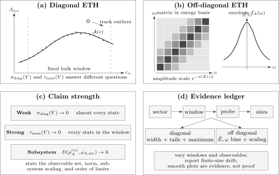
ETH is tested only after resolving a symmetry sector, energy window, observable, and size sequence. Diagonal matrix elements should concentrate around a smooth thermal curve; off-diagonal elements should exhibit an entropy-scaled frequency envelope. Weak and strong claims require different finite-size statistics.

From Diagonal ETH to Thermal Values

Let the initial pure state be

$$|\psi_0\rangle = \sum_n c_n|n\rangle, \qquad p_n=|c_n|^2.$$

After dephasing, the long-time expectation value is

$$\overline{\langle A(t)\rangle} = \sum_n p_n A_{nn}.$$

Insert diagonal ETH:

$$\overline{\langle A(t)\rangle} = \sum_n p_n\mathcal A(E_n) + \sum_n p_n\delta A_{nn}.$$

Define

$$\begin{aligned} \bar E &= \sum_n p_nE_n, \\ (\Delta E)^2 &= \sum_n p_n(E_n-\bar E)^2. \end{aligned}$$

If the occupied energy density is narrow,

$$\frac{\Delta E}{V} \longrightarrow 0,$$

then smoothness permits an expansion about $\bar E$:

$$\begin{aligned} \sum_n p_n\mathcal A(E_n) &= \mathcal A(\bar E) \\ &\quad + \frac{1}{2} \mathcal A''(\bar E) (\Delta E)^2 +\cdots. \end{aligned}$$

The linear term vanishes by definition of $\bar E$. For a local observable whose thermodynamic value is a smooth function of $e=E/V$,

$$\mathcal A''(E) = O(V^{-2}),$$

away from singular points. Thus a subextensive energy width can make the curvature correction vanish.

The ETH fluctuation term obeys the elementary bound

$$\left| \sum_n p_n\delta A_{nn} \right| \le \max_{n:p_n\ne0} |\delta A_{nn}|.$$

Strong ETH makes this small for every narrow-energy preparation in the window. Weak ETH requires an additional condition: the initial state must not place appreciable weight on the rare nonthermal set.

The error ledger

A useful decomposition is

$$\begin{aligned} \overline{\langle A\rangle} - A_{\mathrm{mc}}(\bar E) &= \epsilon_{\mathrm{width}} \\ &\quad + \epsilon_{\mathrm{ETH}} + \epsilon_{\mathrm{shell}}. \end{aligned}$$

Here:

• $\epsilon_{\mathrm{width}}$ measures variation of the smooth function over the occupied energies;
• $\epsilon_{\mathrm{ETH}}$ measures eigenstate fluctuations or rare-state weight;
• $\epsilon_{\mathrm{shell}}$ measures the finite-window convention and finite-size microcanonical error.

Calling a curve “thermal” without separating these errors hides which statement has actually been tested.

From microcanonical to canonical

ETH directly identifies eigenstates with an energy-matched microcanonical prediction. Replacing that prediction by

$$\rho_\beta = \frac{e^{-\beta H}}{Z}$$

requires ensemble equivalence for the chosen observable and thermodynamic regime. ETH alone does not prove canonical–microcanonical equivalence, especially at phase coexistence, for long-range interactions, or for macroscopic observables.

Off-Diagonal ETH and Temporal Fluctuations

The exact time-dependent expectation value is

$$\langle A(t)\rangle = \sum_{m,n} c_m^*c_n e^{i(E_m-E_n)t} A_{mn}.$$

Subtract its dephased value:

$$\delta A(t) = \sum_{m\ne n} c_m^*c_n e^{i(E_m-E_n)t} A_{mn}.$$

If the relevant energy gaps are nondegenerate, the infinite-time variance is

$$\overline{|\delta A(t)|^2} = \sum_{m\ne n} p_mp_n |A_{mn}|^2.$$

Off-diagonal ETH gives the scale

$$|A_{mn}|^2 \sim e^{-S(\bar E)} |f_A(\bar E,\omega)|^2.$$

For a broad, narrow-energy superposition with no anomalously coherent structure, this makes late-time fluctuations exponentially small in system size up to smooth and algebraic factors.

Important qualifications remain:

• degeneracies and repeated gaps alter the time-average formula;
• a small effective dimension can leave large fluctuations;
• special phases among coefficients can create long transients;
• low-frequency hydrodynamic structure can produce slow relaxation;
• recurrence is not removed in a finite spectrum.

ETH is therefore part of a thermalization argument, not a substitute for every dynamical hypothesis.

One Eigenstate Can Be Thermal Without Relaxing

An energy eigenstate evolves only by a phase:

$$e^{-iHt}|n\rangle = e^{-iE_nt}|n\rangle.$$

Its observable expectation value is stationary:

$$\langle n|A(t)|n\rangle = A_{nn}.$$

If diagonal ETH holds, that stationary value is thermal for $A$. There is no relaxation because the state was already locally thermal.

Conversely, a superposition can equilibrate by dephasing even when diagonal ETH fails. It may settle to a nonthermal diagonal ensemble. This is why equilibration and eigenstate thermalization are distinct claims.

Correlations and the Spectral Envelope

The off-diagonal envelope is directly connected to equilibrium correlation functions. For a single eigenstate $|n\rangle$, define the connected correlator

$$C_n(t) = \langle n| A(t)A(0) |n\rangle - A_{nn}^2.$$

Its spectral representation is

$$C_n(t) = \sum_{m\ne n} e^{-i(E_m-E_n)t} |A_{mn}|^2.$$

With

$$C_n(\omega) = \int_{-\infty}^{\infty} dt\, e^{i\omega t} C_n(t),$$

one obtains

$$C_n(\omega) = 2\pi \sum_{m\ne n} |A_{mn}|^2 \delta \left( \omega-E_m+E_n \right).$$

Replacing the nearby-state sum by the density of states and inserting ETH gives, schematically,

$$\begin{aligned} C_n(\omega) &\simeq 2\pi \\ &\quad\times e^{ S(E_n+\omega) - S(E_n+\omega/2) } \\ &\quad\times \left| f_A(E_n+\omega/2,\omega) \right|^2. \end{aligned}$$

For $\omega$ small on thermodynamic scales,

$$S(E_n+\omega) - S(E_n+\omega/2) \simeq \frac{\beta\omega}{2},$$

so

$$C_n(\omega) \simeq 2\pi e^{\beta\omega/2} |f_A(E_n,\omega)|^2.$$

For Hermitian $A$ and the corresponding envelope symmetry,

$$\frac{C_n(-\omega)}{C_n(\omega)} \simeq e^{-\beta\omega}.$$

This is the eigenstate-level origin of thermal detailed balance. Exact conventions depend on Fourier signs, entropy coarse graining, and whether a connected or symmetrized correlator is used. Time-Dependent Correlations, Spectral Functions, and the Fluctuation–Dissipation Theorem own those conventions and consequences.

Pairwise ETH is not the whole dynamics

The standard ansatz controls one- and two-eigenstate data: diagonal values and pairwise matrix elements. Operator spreading, entanglement growth, out-of-time-order correlators, and other higher-point quantities can depend on correlations among four or more eigenstates.

Thus:

$$\begin{gathered} \text{standard ETH} \centernot\Longrightarrow \\ \text{complete statistics of chaotic dynamics}. \end{gathered}$$

Modern extensions study these multi-eigenstate correlations. Many-Body Quantum Chaos Preview and Scrambling and OTOCs Preview own that frontier.

Subsystem ETH

Let the system factor as

$$\mathcal H = \mathcal H_A\otimes\mathcal H_B,$$

and define an eigenstate reduced density operator

$$\rho_A^{(n)} = \operatorname{Tr}_B |n\rangle\langle n|.$$

The reduced microcanonical state is

$$\rho_{A,\mathrm{mc}} = \operatorname{Tr}_B \rho_{\mathrm{mc}}.$$

Subsystem ETH asks, under specified scaling of $A$ relative to the full system, that

$$D\left( \rho_A^{(n)}, \rho_{A,\mathrm{mc}} \right) \longrightarrow 0,$$

where

$$D(\rho,\sigma) = \frac12 \|\rho-\sigma\|_1.$$

This is stronger than agreement for one observable. It implies agreement for every bounded measurement confined to subsystem $A$:

$$\begin{aligned} & \left| \operatorname{Tr} \left[ O_A \left( \rho_A^{(n)} - \rho_{A,\mathrm{mc}} \right) \right] \right| \\ &\qquad\le 2 \|O_A\|_\infty D\left( \rho_A^{(n)}, \rho_{A,\mathrm{mc}} \right). \end{aligned}$$

The subsystem limit matters

The cleanest formulation holds for fixed subsystem size while

$$V\to\infty.$$

If

$$f = \frac{V_A}{V}$$

remains finite, global purity, energy conservation, and complement constraints matter at leading or subleading order. A half-system reduced state is not governed by the same approximation as a fixed local region.

Subsystem ETH can imply a volume-law eigenstate entanglement entropy with thermal leading coefficient. That derivation belongs to Thermal Entropy versus Entanglement Entropy and Volume Laws.

ETH, Typicality, and Ensemble Equivalence

Three statements are often blended together:

Canonical typicality

Most randomly sampled pure states in a high-dimensional constrained shell are locally close to the shell state.

Eigenstate thermalization

The specially selected vectors that diagonalize a physical Hamiltonian are locally thermal and have structured matrix elements.

Ensemble equivalence

Different mixed equilibrium ensembles give the same predictions for a declared observable class in a thermodynamic limit.

None follows from the definition of another. Their conclusions can coincide in generic systems, but their measures, assumptions, and failure modes differ.

A Concrete Diagnostic Model

A standard nonintegrable testbed is the mixed-field Ising chain

$$\begin{aligned} H &= J \sum_{j=1}^{L-1} Z_jZ_{j+1} \\ &\quad+ h_x \sum_{j=1}^{L} X_j \\ &\quad+ h_z \sum_{j=1}^{L} Z_j. \end{aligned}$$

With generic nonzero $h_x$ and $h_z$, the longitudinal field breaks the spin-flip symmetry that makes the transverse-field model integrable. Open uniform boundaries retain reflection symmetry, so reflection sectors must still be separated.

Possible probes include

$$A_1 = Z_{\lfloor L/2\rfloor}, \qquad A_2 = Z_{\lfloor L/2\rfloor} Z_{\lfloor L/2\rfloor+1},$$

and the intensive energy-density components

$$A_3 = \frac{1}{L} \sum_j X_j.$$

The Transverse-Field Ising Model owns the integrable limit and its exact structure. Here the mixed-field deformation is only a diagnostic laboratory.

How to Test Diagonal ETH

1. Resolve all exact symmetries

Block diagonalize by particle number, momentum, parity, reflection, or other exact labels. Document whether the observable preserves or connects those sectors.

2. Choose energy-density windows

Use a window centered at fixed

$$e = \frac{E}{L}$$

as $L$ varies. Report both $\Delta E$ and the number of states $D_{\mathcal W}$.

3. Plot eigenstate expectation values

Plot

$$A_{nn} \quad\text{against}\quad e_n=\frac{E_n}{L}.$$

In an ETH regime, the cloud narrows around a smooth curve in the spectral bulk. Visual smoothness is orientation, not a scaling result.

4. Subtract a local smooth benchmark

Define a local shell estimate

$$\widehat{\mathcal A}_L(E_n) = \frac{1}{N_n} \sum_{ m: |E_m-E_n|<\Delta/2 } A_{mm}.$$

Then analyze residuals

$$\delta A_{nn}^{(L)} = A_{nn} - \widehat{\mathcal A}_L(E_n).$$

The smoothing width must contain many levels but resolve thermodynamic variation. Vary it as a robustness check.

5. Track both typical and extreme statistics

Useful diagnostics include

$$\sigma_{\mathrm{diag}}^2(L) = \frac{1}{D_{\mathcal W}} \sum_{n\in\mathcal W} \left| \delta A_{nn}^{(L)} \right|^2,$$

the median absolute deviation,

$$\operatorname{MAD}(L) = \operatorname{median}_{n\in\mathcal W} \left| \delta A_{nn}^{(L)} \right|,$$

and the maximum

$$r_{\max}(L) = \max_{n\in\mathcal W} \left| \delta A_{nn}^{(L)} \right|.$$

The variance probes weak ETH. The maximum probes strong ETH and is much more sensitive to rare states and finite-size drift.

6. Inspect the full distribution

A shrinking variance can coexist with long tails. Report quantiles or the empirical distribution

$$P_L(\delta A)$$

instead of compressing every result to one number.

How to Test Off-Diagonal ETH

For each pair $m\ne n$, bin matrix elements by

$$\bar E = \frac{E_m+E_n}{2}$$

and

$$\omega = E_m-E_n.$$

Within a narrow bin, estimate

$$\overline{|A_{mn}|^2}_{\bar E,\omega}.$$

The entropy-rescaled variance is

$$\mathcal F_A(\bar E,\omega) = e^{S(\bar E)} \overline{|A_{mn}|^2}_{\bar E,\omega}.$$

ETH predicts that $\mathcal F_A$ approaches a smooth function proportional to $|f_A|^2$.

Distribution tests

Define rescaled elements

$$\widetilde R_{mn} = \frac{ e^{S(\bar E)/2}A_{mn} }{ \sqrt{\mathcal F_A(\bar E,\omega)} }.$$

One can test:

• zero mean;
• unit variance;
• real or complex distribution appropriate to symmetries;
• higher moments;
• correlations between neighboring matrix elements.

Approximate Gaussianity is common in random-matrix-like regimes, but it is not the entire ETH content and need not hold at every frequency.

Low-frequency structure

Near $\omega=0$, transport and conservation laws can dominate. A diffusive density produces long timescales and a narrow spectral structure. The entries $R_{mn}$ cannot then be treated as independent down to arbitrary energy scales.

This is not a failure of thermodynamics. It is evidence that the spectral envelope and matrix-element correlations remember locality and hydrodynamics.

Exact Toy Example: Weak ETH Without Strong ETH

Consider a shell containing $D$ eigenstates. Let

$$A_{nn} = a$$

for $D-1$ states and

$$A_{**} = a+\delta$$

for one exceptional state $|*\rangle$, with $\delta$ independent of $D$.

The shell mean is

$$A_{\mathrm{mc}} = a+\frac{\delta}{D}.$$

The variance is

$$\begin{aligned} \sigma_{A,\mathrm{mc}}^2 &= \frac{D-1}{D} \left( \frac{\delta}{D} \right)^2 \\ &\quad + \frac{1}{D} \left[ \delta \left( 1-\frac{1}{D} \right) \right]^2, \end{aligned}$$

so

$$\sigma_{A,\mathrm{mc}}^2 = \delta^2 \frac{D-1}{D^2} \longrightarrow 0.$$

Weak ETH holds. But

$$r_{\max} = |\delta| \left( 1-\frac{1}{D} \right) \longrightarrow |\delta|,$$

so strong ETH fails.

Now choose an initial state with probability $p_*$ on the exceptional eigenstate. Its diagonal expectation is

$$\overline{\langle A\rangle} = a+p_*\delta.$$

If $p_*$ remains order one, the state stays nonthermal even though almost every shell eigenstate is thermal. Weak ETH is a typical-state statement, not protection against adversarial preparation.

When ETH Fails or Needs Qualification

Integrability

Integrable systems possess extensively many conserved quantities. Eigenstate expectation values can depend on the corresponding charge densities, so energy alone does not label the local thermodynamic macrostate. Ordinary Gibbs ETH fails, although generalized eigenstate statements may hold after all relevant charges are fixed.

Integrability and Generalized Gibbs Ensembles Preview owns generalized stationary ensembles and their relation to the conserved-charge hierarchy.

Many-body localization

An idealized many-body localized phase has quasilocal integrals of motion, persistent local memory, and nonthermal highly excited eigenstates. Local observables can vary strongly between nearby energies, and eigenstate entanglement can obey an area law rather than a thermal volume law.

Many-Body Localization Preview owns the evidence, stability questions, and finite-size caveats.

Hilbert-space fragmentation

Kinetic or gauge constraints can split a formal symmetry sector into dynamically disconnected Krylov sectors:

$$\mathcal H_q = \bigoplus_\alpha \mathcal K_{q,\alpha}.$$

An ETH-like statement may hold inside each sufficiently large component while failing across their union. The accessible component is part of the conserved information.

Rare embedded eigenstates and scars

Local translationally invariant Hamiltonians can be constructed with a small set of exact nonthermal eigenstates embedded in an otherwise thermal spectrum. Quantum many-body scars provide physically important families of atypical low-entanglement eigenstates and can support revivals from specially chosen initial states.

Such systems can satisfy weak ETH while violating strong ETH. They also show that strong ETH is sufficient but not logically necessary for thermalization of most experimentally generic initial states.

Symmetry breaking and phase coexistence

Finite systems with an exact symmetry can have cat-like eigenstates even where thermodynamic pure phases break that symmetry. Order parameters, boundary conditions, sector projections, and the order of limits must be handled together.

Near first-order thermal transitions, multiple macroscopic branches can coexist at similar energy density. A single smooth function $\mathcal A(E)$ may be an inadequate finite-size description until the phase label and limiting prescription are specified.

Spectral edges and low-energy states

ETH is primarily a finite-energy-density statement. Ground states, topological sectors, quasiparticles above a vacuum, and low-entropy spectral edges need not resemble thermal bulk eigenstates.

Nonlocal and state-selective observables

Projectors onto eigenstates, Wilson-loop-scale probes, global order parameters, and operators whose support grows with system size can retain information invisible to local observables. The observable support and normalization must accompany the claim.

Long-range interactions

For slowly decaying interactions, conventional locality bounds, additivity, ensemble equivalence, and finite-size scaling can change. One should not import short-range ETH scaling without checking the interaction exponent and thermodynamic normalization.

Relation to Quantum Chaos

ETH and quantum chaos are deeply connected but not interchangeable.

Quantum-chaos diagnostics include:

• level repulsion within an irreducible sector;
• random-matrix spectral correlations;
• eigenvector delocalization in physically motivated bases;
• operator growth and scrambling;
• spectral form factors.

ETH concerns matrix elements of specified observables. Level statistics can indicate a chaotic regime while a chosen observable retains slow hydrodynamic structure. Conversely, selected ETH-like statements can hold in settings where standard spectral diagnostics are subtle.

The safe implication is empirical and model dependent:

$$\begin{gathered} \text{generic nonintegrable regime} \\ \Longrightarrow \\ \text{often chaotic spectral statistics} \\ \text{and ETH behavior} \end{gathered}$$

but

$$\text{one diagnostic} \centernot\Longleftrightarrow \text{the other}.$$

Many-Body Quantum Chaos Preview owns level statistics, random-matrix ensembles, Thouless scales, and their limitations.

What Experiments Can Test

Directly preparing and comparing many individual many-body eigenstates is difficult. Experiments more often test consequences compatible with ETH:

• local observables approach energy-matched ensemble values;
• different initial states with the same conserved densities approach the same local predictions;
• small subsystems acquire thermal reduced states while the global state remains pure;
• entanglement entropy approaches a thermal volume-law value;
• integrability breaking changes stationary behavior;
• rare preparations exhibit anomalous revivals or memory.

Quantum-gas microscopy experiments have reconstructed local reduced states and entanglement in small isolated systems, finding local thermal behavior compatible with ETH while preserving global purity. Superconducting-qubit experiments have similarly explored entanglement and ergodic dynamics in controlled few-qubit systems.

These observations support the ETH framework in particular models. They do not establish a universal theorem for all macroscopic Hamiltonians.

What Is Established and What Is Not

Established

• ETH provides a precise and highly successful framework for many generic nonintegrable lattice models.
• Diagonal smoothness explains initial-state-independent thermal values for narrow-energy preparations.
• Off-diagonal entropy scaling is well supported numerically for many local observables.
• Weak ETH has rigorous support under broad assumptions in several settings.
• Integrability, localization, fragmentation, and scars provide controlled failure mechanisms.

Not universal

• Strong ETH is not valid for every local nonintegrable Hamiltonian.
• Nonintegrability alone is not a proof of ETH.
• Random-matrix independence is not valid at all frequencies or for all matrix-element correlations.
• ETH does not determine a universal relaxation time.
• Standard ETH does not fully determine scrambling or higher-point quantum-information dynamics.

Active refinements

Research continues on:

• the strongest general conditions implying weak or strong ETH;
• rare-state large deviations;
• hydrodynamic constraints on low-frequency matrix elements;
• higher-order eigenstate correlations;
• subsystem fractions that scale with total size;
• long-range, constrained, gauge, and field-theory settings.

These refinements do not undermine the standard ETH framework. They specify its resolution and domain.

Common Mistakes

• Calling ETH a theorem for every nonintegrable system. It is a hypothesis with extensive support and explicit counterexamples.
• Mixing symmetry sectors. ETH and chaos diagnostics must be sector resolved.
• Testing only one system size. ETH is a thermodynamic scaling claim.
• Using a visual EEV cloud as proof. Quantify width, tails, outliers, and window dependence.
• Equating weak and strong ETH. Vanishing variance does not control the worst eigenstate.
• Ignoring the initial state’s rare-state weight. Weak ETH does not guarantee every preparation thermalizes.
• Treating $R_{mn}$ as literally independent noise. Hermiticity, conservation, locality, transport, and higher-point correlations constrain it.
• Demanding ETH for arbitrary projectors. The observable class is essential.
• Replacing microcanonical by canonical without checking equivalence. That is a separate thermodynamic step.
• Equating an eigenstate with a global Gibbs state. Agreement is local or observable restricted.
• Inferring a relaxation time from $e^{-S/2}$. The frequency envelope and conserved slow modes determine timescales.
• Using level repulsion as an ETH proof. Spectral and matrix-element diagnostics answer related but different questions.
• Taking a fixed finite-size outlier as a thermodynamic violation. Its scaling with size is the relevant evidence.
• Discarding rare states because they are few. Special preparations can concentrate on them.

Exercises

1. Sector mixing can mimic ETH failure

Suppose a Hamiltonian has two exact sectors, $q=\pm1$. In a narrow energy window, an observable commuting with the symmetry has

$$A_{nn} \simeq \begin{cases} a+\delta,&q=+1,\\ a-\delta,&q=-1. \end{cases}$$

Assume each sector separately has vanishing within-sector variance and contains the same number of states. Compute the variance obtained by pooling the sectors. Does it vanish?

Solution

The pooled mean is

$$A_{\mathrm{pool}} = a.$$

Neglecting the vanishing within-sector variances, every state differs from the pooled mean by magnitude $|\delta|$. Therefore

$$\sigma_{\mathrm{pool}}^2 = \delta^2.$$

It does not vanish. The pooled data falsely suggest ETH failure even though each irreducible sector satisfies diagonal ETH. Sector resolution is part of the definition, not optional preprocessing.

2. Motivate the entropy factor

A microcanonical shell has dimension $D=e^S$. A bounded local observable satisfies

$$\frac{1}{D} \operatorname{Tr}_{\mathcal W} (A^\dagger A) = c$$

with $c=O(1)$. Assume its off-diagonal Hilbert–Schmidt weight is distributed over order $D^2$ entries. Estimate the typical magnitude of $A_{mn}$ for $m\ne n$.

Solution

The trace identity gives

$$\sum_{m,n\in\mathcal W} |A_{mn}|^2 = cD.$$

If order $D^2$ entries carry comparable off-diagonal weight, then

$$\overline{|A_{mn}|^2} \sim \frac{cD}{D^2} = \frac{c}{D}.$$

Thus

$$|A_{mn}|_{\mathrm{typ}} \sim \sqrt c\,D^{-1/2} = \sqrt c\,e^{-S/2}.$$

This estimates the scale but does not establish the smooth envelope or statistical independence.

3. Energy-width correction

Let a local thermal value depend smoothly on energy density:

$$\mathcal A(E) = g\left(\frac{E}{V}\right).$$

Show that the leading width correction for a state centered at $\bar E$ is

$$\frac{g''(\bar e)}{2} \frac{(\Delta E)^2}{V^2}, \qquad \bar e=\frac{\bar E}{V}.$$

What condition makes it vanish?

Solution

Differentiating with respect to total energy,

$$\mathcal A'(E) = \frac{1}{V} g'\left(\frac{E}{V}\right),$$

and

$$\mathcal A''(E) = \frac{1}{V^2} g''\left(\frac{E}{V}\right).$$

The linear term averages to zero because

$$\sum_n p_n(E_n-\bar E)=0.$$

Hence the leading correction is

$$\frac12 \mathcal A''(\bar E) (\Delta E)^2 = \frac{g''(\bar e)}{2} \frac{(\Delta E)^2}{V^2}.$$

It vanishes when $\Delta E/V\to0$ and $g''$ remains finite.

4. One outlier

For the toy shell with $D-1$ values equal to $a$ and one value equal to $a+\delta$, calculate the bad-state fraction for any tolerance satisfying

$$0<\epsilon<|\delta|.$$

Compare it with the maximum deviation as $D\to\infty$.

Solution

For sufficiently large $D$, only the exceptional state differs from the shell mean by more than $\epsilon$. Thus

$$f_{\mathrm{bad}}(\epsilon) = \frac{1}{D} \longrightarrow 0.$$

Meanwhile,

$$r_{\max} \longrightarrow |\delta|.$$

The example satisfies weak ETH but violates strong ETH.

5. Temporal variance from off-diagonal ETH

Assume nondegenerate energy gaps and a state with probabilities $p_n$. Starting from

$$\delta A(t) = \sum_{m\ne n} c_m^*c_n e^{i(E_m-E_n)t} A_{mn},$$

derive the infinite-time variance. Then use

$$|A_{mn}|^2 \le C e^{-S_*}$$

throughout the occupied window to bound it.

Solution

Multiplying by the complex conjugate produces terms labeled by two energy gaps. Nondegenerate gaps make all unequal-gap terms vanish under infinite-time averaging, leaving

$$\overline{|\delta A(t)|^2} = \sum_{m\ne n} p_mp_n |A_{mn}|^2.$$

Using the bound,

$$\overline{|\delta A(t)|^2} \le C e^{-S_*} \sum_{m\ne n} p_mp_n.$$

Since

$$\sum_{m\ne n}p_mp_n = 1-\sum_n p_n^2 \le 1,$$

one obtains

$$\overline{|\delta A(t)|^2} \le C e^{-S_*}.$$

The assumptions exclude gap degeneracies and anomalous low-frequency matrix elements.

6. Subsystem ETH and measurements

Suppose

$$D\left( \rho_A^{(n)}, \rho_{A,\mathrm{mc}} \right) \le \varepsilon.$$

Bound the difference in expectation values of a Hermitian observable $O_A$ with

$$\|O_A\|_\infty\le1.$$

Solution

Trace-norm duality gives

$$\begin{aligned} & \left| \operatorname{Tr} \left[ O_A \left( \rho_A^{(n)} - \rho_{A,\mathrm{mc}} \right) \right] \right| \\ &\qquad\le \|O_A\|_\infty \left\| \rho_A^{(n)} - \rho_{A,\mathrm{mc}} \right\|_1. \end{aligned}$$

Because trace distance is half the trace norm,

$$\left\| \rho_A^{(n)} - \rho_{A,\mathrm{mc}} \right\|_1 \le 2\varepsilon.$$

Therefore the expectation-value difference is at most $2\varepsilon$.

7. Detailed balance from the ETH envelope

Assume

$$C_n(\omega) \simeq 2\pi e^{\beta\omega/2} |f_A(E_n,\omega)|^2$$

and

$$|f_A(E,-\omega)|^2 = |f_A(E,\omega)|^2.$$

Derive the detailed-balance ratio.

Solution

Replacing $\omega$ by $-\omega$ gives

$$C_n(-\omega) \simeq 2\pi e^{-\beta\omega/2} |f_A(E_n,\omega)|^2.$$

Dividing,

$$\frac{C_n(-\omega)}{C_n(\omega)} \simeq e^{-\beta\omega}.$$

The result uses the chosen Fourier convention. Reversing the convention reverses which spectrum appears in the numerator.

8. Design an ETH test

Design a finite-size ETH study for the mixed-field Ising chain. State at least six checks required before claiming strong ETH for a local spin observable.

Solution

A credible study would:

1. specify $J$, $h_x$, $h_z$, boundaries, and the sequence of lengths $L$;
2. resolve reflection and every other exact symmetry;
3. choose a bulk window at fixed energy density and report its level count;
4. define the local observable and its normalization;
5. subtract a documented smooth microcanonical benchmark;
6. report both typical width and maximum deviation versus $L$;
7. vary the smoothing and shell widths;
8. inspect residual distributions and outliers rather than only their variance;
9. compare more than one local observable;
10. separate diagonal from off-diagonal tests.

Strong ETH requires evidence that the maximum deviation tends to zero, not merely that most points form a narrow cloud.

Further Connections

• Nonequilibrium Overview places ETH among quench, integrability, localization, and driving mechanisms.
• Quantum Quenches defines the initial-state energy distribution to which diagonal ETH is applied.
• Relaxation and Thermalization separates dephasing error from ensemble-identification error.
• Microcanonical Ensemble defines the shell average used in every diagonal test.
• Ensemble Equivalence controls the later replacement of microcanonical by canonical predictions.
• Time-Dependent Correlations develops the spectral data encoded by the off-diagonal envelope.
• Thermal Entropy versus Entanglement Entropy owns the reduced-state and entropy consequences.

Summary

The eigenstate thermalization hypothesis is a structured claim about simple operators in the energy eigenbasis:

$$A_{mn} = \mathcal A(\bar E)\delta_{mn} + e^{-S(\bar E)/2} f_A(\bar E,\omega)R_{mn}.$$

Its diagonal part says that nearby eigenstates are locally indistinguishable and therefore reproduce microcanonical values. Its off-diagonal part suppresses temporal fluctuations and encodes equilibrium spectral response. Weak ETH controls almost all eigenstates; strong ETH controls the worst outlier; subsystem ETH controls every measurement on a declared region.

A trustworthy ETH claim always names the sector, window, observable, norm, size sequence, and order of limits. Integrability, localization, fragmentation, scars, spectral edges, nonlocal probes, and conserved slow modes are not footnotes: they define the boundary of the hypothesis.

References

1. J. M. Deutsch, “Quantum statistical mechanics in a closed system,” Physical Review A 43, 2046–2049 (1991). doi:10.1103/PhysRevA.43.2046
2. M. Srednicki, “Chaos and quantum thermalization,” Physical Review E 50, 888–901 (1994). doi:10.1103/PhysRevE.50.888
3. M. Srednicki, “The approach to thermal equilibrium in quantized chaotic systems,” Journal of Physics A: Mathematical and General 32, 1163–1175 (1999). doi:10.1088/0305-4470/32/7/007
4. M. Rigol, V. Dunjko, and M. Olshanii, “Thermalization and its mechanism for generic isolated quantum systems,” Nature 452, 854–858 (2008). doi:10.1038/nature06838
5. M. Rigol and M. Srednicki, “Alternatives to eigenstate thermalization,” Physical Review Letters 108, 110601 (2012). doi:10.1103/PhysRevLett.108.110601
6. A. Polkovnikov, K. Sengupta, A. Silva, and M. Vengalattore, “Colloquium: Nonequilibrium dynamics of closed interacting quantum systems,” Reviews of Modern Physics 83, 863–883 (2011). doi:10.1103/RevModPhys.83.863
7. L. D’Alessio, Y. Kafri, A. Polkovnikov, and M. Rigol, “From quantum chaos and eigenstate thermalization to statistical mechanics and thermodynamics,” Advances in Physics 65, 239–362 (2016). doi:10.1080/00018732.2016.1198134
8. J. M. Deutsch, “Eigenstate thermalization hypothesis,” Reports on Progress in Physics 81, 082001 (2018). doi:10.1088/1361-6633/aac9f1
9. P. Reimann, “Eigenstate thermalization: Deutsch’s approach and beyond,” New Journal of Physics 17, 055025 (2015). doi:10.1088/1367-2630/17/5/055025
10. T. Mori, T. N. Ikeda, E. Kaminishi, and M. Ueda, “Thermalization and prethermalization in isolated quantum systems: a theoretical overview,” Journal of Physics B 51, 112001 (2018). doi:10.1088/1361-6455/aabcdf
11. C. Gogolin and J. Eisert, “Equilibration, thermalisation, and the emergence of statistical mechanics in closed quantum systems,” Reports on Progress in Physics 79, 056001 (2016). doi:10.1088/0034-4885/79/5/056001
12. L. F. Santos and M. Rigol, “Localization and the effects of symmetries in the thermalization properties of one-dimensional quantum systems,” Physical Review E 82, 031130 (2010). doi:10.1103/PhysRevE.82.031130
13. T. N. Ikeda, Y. Watanabe, and M. Ueda, “Finite-size scaling analysis of the eigenstate thermalization hypothesis in a one-dimensional interacting Bose gas,” Physical Review E 87, 012125 (2013). doi:10.1103/PhysRevE.87.012125
14. R. Steinigeweg, J. Herbrych, and P. Prelovšek, “Eigenstate thermalization within isolated spin-chain systems,” Physical Review E 87, 012118 (2013). doi:10.1103/PhysRevE.87.012118
15. W. Beugeling, R. Moessner, and M. Haque, “Finite-size scaling of eigenstate thermalization,” Physical Review E 89, 042112 (2014). doi:10.1103/PhysRevE.89.042112
16. W. Beugeling, R. Moessner, and M. Haque, “Off-diagonal matrix elements of local operators in many-body quantum systems,” Physical Review E 91, 012144 (2015). doi:10.1103/PhysRevE.91.012144
17. H. Kim, T. N. Ikeda, and D. A. Huse, “Testing whether all eigenstates obey the eigenstate thermalization hypothesis,” Physical Review E 90, 052105 (2014). doi:10.1103/PhysRevE.90.052105
18. G. Biroli, C. Kollath, and A. M. Läuchli, “Effect of rare fluctuations on the thermalization of isolated quantum systems,” Physical Review Letters 105, 250401 (2010). doi:10.1103/PhysRevLett.105.250401
19. N. Shiraishi and T. Mori, “Systematic construction of counterexamples to the eigenstate thermalization hypothesis,” Physical Review Letters 119, 030601 (2017). doi:10.1103/PhysRevLett.119.030601
20. A. Dymarsky, N. Lashkari, and H. Liu, “Subsystem eigenstate thermalization hypothesis,” Physical Review E 97, 012140 (2018). doi:10.1103/PhysRevE.97.012140
21. P. Reimann, “Dynamical typicality approach to eigenstate thermalization,” Physical Review Letters 120, 230601 (2018). doi:10.1103/PhysRevLett.120.230601
22. A. Dymarsky, “Bound on eigenstate thermalization from transport,” Physical Review Letters 128, 190601 (2022). doi:10.1103/PhysRevLett.128.190601
23. C. J. Turner, A. A. Michailidis, D. A. Abanin, M. Serbyn, and Z. Papić, “Weak ergodicity breaking from quantum many-body scars,” Nature Physics 14, 745–749 (2018). doi:10.1038/s41567-018-0137-5
24. R. Nandkishore and D. A. Huse, “Many-body localization and thermalization in quantum statistical mechanics,” Annual Review of Condensed Matter Physics 6, 15–38 (2015). doi:10.1146/annurev-conmatphys-031214-014726
25. A. M. Kaufman, M. E. Tai, A. Lukin, M. Rispoli, R. Schittko, P. M. Preiss, and M. Greiner, “Quantum thermalization through entanglement in an isolated many-body system,” Science 353, 794–800 (2016). doi:10.1126/science.aaf6725
26. C. Neill, P. Roushan, M. Fang, et al., “Ergodic dynamics and thermalization in an isolated quantum system,” Nature Physics 12, 1037–1041 (2016). doi:10.1038/nphys3830
27. D. Hahn, D. J. Luitz, and J. T. Chalker, “Eigenstate correlations, the eigenstate thermalization hypothesis, and quantum information dynamics in chaotic many-body quantum systems,” Physical Review X 14, 031029 (2024). doi:10.1103/PhysRevX.14.031029