Thermal Entropy vs Entanglement Entropy

Thermal entropy and entanglement entropy are computed with the same von Neumann formula, but they answer different physical questions. Thermal entropy describes the mixedness of an equilibrium state under specified macroscopic constraints. Entanglement entropy describes correlations across a bipartition when the joint state is pure. A subsystem of a pure many-body state can nevertheless look thermal, so the two quantities may agree locally and even share a leading volume-law coefficient without becoming conceptually identical.

The safest first question is not “What is the entropy?” It is:

$$\begin{gathered} \text{Which density operator} \\ \text{is being assigned an entropy,} \\ \text{and what larger state or ensemble} \\ \text{produced it?} \end{gathered}$$

This page develops an entropy ledger that keeps the total state, the subsystem, the ensemble, and the scaling limit visible at every step. It explains exact equalities, controlled approximations, and misleading coincidences among:

• the thermodynamic entropy of a mixed Gibbs or microcanonical state;
• the entanglement entropy of a subsystem of a globally pure state;
• the ordinary subsystem entropy of a globally mixed state;
• the thermal-like entropy of a small region in a typical pure state or a thermalizing eigenstate;
• volume laws in thermal states, random pure states, excited eigenstates, and post-quench states.

Scope and Canonical Ownership

This page is the canonical home for the direct comparison between thermal entropy and many-body entanglement entropy. It owns:

• a state-by-state entropy ledger based on global purity and subsystem reduction;
• exact comparisons among pure entangled states, mixed thermal states, and purifications;
• why a thermal volume law is not automatically entanglement;
• why a pure state can have thermal-like reduced density operators;
• canonical typicality and the reduced-state form of eigenstate thermalization at overview depth;
• the subsystem-fraction and full-system endpoint tests;
• the distinction between von Neumann and Rényi comparisons in extensive subsystems;
• finite-size, ensemble, conservation-law, and order-of-limits cautions.

Nearby pages retain their canonical roles:

• Entropy in Quantum Statistical Mechanics owns Gibbs, microcanonical, grand-canonical, diagonal, and coarse-grained entropy identities.
• Entanglement Entropy owns the finite-dimensional pure-state entanglement measure.
• Subsystem Entropy owns the general interpretation of local mixedness.
• Entanglement Entropy in Many-Body Systems owns spatial scaling laws, continuum divergences, numerical extraction, and phase diagnostics.
• Many-Body Entanglement Overview owns the chapter-wide partition, state-class, measure, and scaling workflow.

The discussion below uses those results rather than rederiving every general property. The Many-Body Entanglement Glossary gives the quick purity, entropy, mutual-information, and Page-curve lookup.

Convention Ledger

Dimensionless and physical entropy

Write

$$\mathcal S(\rho) := -\operatorname{Tr} \left( \rho\ln\rho \right)$$

for dimensionless von Neumann entropy in nats. Thermodynamic entropy carries Boltzmann’s constant:

$$S_{\mathrm{th}} = k_{\mathrm B}\mathcal S(\rho_{\mathrm{eq}}).$$

This separation prevents a silent factor of $k_{\mathrm B}$ from entering pure-state entanglement calculations. Divide $\mathcal S$ by $\ln2$ to obtain bits.

Total system and subsystem

The total finite system is denoted

$$X=AB, \qquad \mathcal H_X \cong \mathcal H_A\otimes\mathcal H_B.$$

For a state $\rho_{AB}$,

$$\rho_A = \operatorname{Tr}_B\rho_{AB}, \qquad \rho_B = \operatorname{Tr}_A\rho_{AB}.$$

We abbreviate

$$\mathcal S_A = \mathcal S(\rho_A), \qquad \mathcal S_{AB} = \mathcal S(\rho_{AB}).$$

In lattice applications, $V_A$ and $V_B$ count sites or physical volume, $V=V_A+V_B$, and

$$f := \frac{V_A}{V}$$

is the subsystem fraction.

Thermal states

For a Hamiltonian $H$ at inverse temperature

$$\beta = \frac{1}{k_{\mathrm B}T},$$

the canonical state is

$$\rho_\beta = \frac{e^{-\beta H}}{Z(\beta)}, \qquad Z(\beta) = \operatorname{Tr}e^{-\beta H}.$$

The phrase “thermal entropy” will mean the thermodynamic entropy assigned to an equilibrium ensemble under specified constraints. The ensemble and conserved quantities must be stated.

Pure-state entanglement

When

$$\rho_{AB} = \lvert\Psi\rangle\langle\Psi\rvert$$

is pure, $\mathcal S_A$ is the entanglement entropy across $A\vert B$. When $\rho_{AB}$ is mixed, $\mathcal S_A$ is only a subsystem entropy; it is not a general mixed-state entanglement measure.

One Formula, Three Questions

State entropy

The expression $\mathcal S(\rho)$ first measures the spectral mixedness of the particular density operator $\rho$. It vanishes exactly for a pure state:

$$\mathcal S(\rho)=0 \quad\Longleftrightarrow\quad \rho^2=\rho$$

in finite dimension.

That mathematical fact does not identify why $\rho$ is mixed. The mixedness may arise from:

• an equilibrium ensemble;
• discarding a complement;
• classical uncertainty in preparation;
• coupling to an unobserved environment;
• deliberate coarse graining;
• averaging over outcomes or disorder.

Subsystem entropy

The entropy $\mathcal S_A$ concerns the reduced state visible to observers restricted to $A$. It can be nonzero even when the total state is pure:

$$\mathcal S_{AB}=0, \qquad \mathcal S_A>0.$$

In that case, all local mixedness comes from entanglement with $B$. If the total state is mixed, local mixedness has more than one possible source.

Thermodynamic entropy

For an equilibrium Gibbs state,

$$\begin{aligned} \mathcal S(\rho_\beta) &= -\operatorname{Tr} \left[ \rho_\beta \left( -\beta H-\ln Z \right) \right] \\ &= \beta\langle H\rangle_\beta +\ln Z. \end{aligned}$$

With Helmholtz free energy

$$F = -\frac{1}{\beta}\ln Z,$$

this becomes

$$S_{\mathrm{th}} = k_{\mathrm B}\beta \left( E-F \right).$$

This identity belongs to equilibrium statistical mechanics. The same trace formula applied to a reduced pure state has a different physical interpretation.

The Exact Entropy Ledger

Globally pure state

Let

$$\lvert\Psi\rangle_{AB} = \sum_{\alpha=1}^{r} \sqrt{\lambda_\alpha} \lvert\alpha\rangle_A \lvert\alpha\rangle_B$$

be a Schmidt decomposition. Then

$$\mathcal S_{AB}=0$$

and

$$\mathcal S_A = \mathcal S_B = -\sum_{\alpha=1}^{r} \lambda_\alpha\ln\lambda_\alpha.$$

This equality is exact at every finite size. It implies complement symmetry:

$$\mathcal S_A = \mathcal S_B.$$

For a pure state, therefore, reduced entropy is entirely entanglement across the chosen cut.

Globally mixed state

For a mixed $\rho_{AB}$, no equality requires $\mathcal S_A=\mathcal S_B$. The universal bounds are

$$\left| \mathcal S_A-\mathcal S_B \right| \le \mathcal S_{AB} \le \mathcal S_A+\mathcal S_B.$$

The right inequality is subadditivity; the left inequality is the Araki–Lieb inequality.

Define quantum mutual information by

$$I(A:B) := \mathcal S_A +\mathcal S_B -\mathcal S_{AB}.$$

It obeys

$$I(A:B)\ge0$$

and vanishes exactly for a product state:

$$I(A:B)=0 \quad\Longleftrightarrow\quad \rho_{AB} = \rho_A\otimes\rho_B.$$

For a pure state,

$$I(A:B) = 2\mathcal S_A.$$

For a mixed state, mutual information measures total correlation, classical and quantum together. It is often a better first audit than $\mathcal S_A$ because it subtracts independent local mixedness.

Conditional entropy as a one-way witness

The conditional entropy is

$$\mathcal S(A|B) := \mathcal S_{AB}-\mathcal S_B.$$

For a pure entangled state,

$$\mathcal S(A|B) = -\mathcal S_A<0.$$

For a product mixed state,

$$\mathcal S(A|B) = \mathcal S_A\ge0.$$

Negative quantum conditional entropy certifies entanglement, but nonnegative conditional entropy does not prove separability. It is a sufficient witness, not a complete mixed-state entanglement test.

Four-state decision table

Global state	$\mathcal S_{AB}$	Meaning of $\mathcal S_A$	Useful companion diagnostic
pure product	$0$	zero across this cut	factorization
pure entangled	$0$	entanglement entropy	Schmidt spectrum, $I=2\mathcal S_A$
mixed product thermal	$>0$	local thermal mixing	$I=0$
mixed correlated thermal	$>0$	thermal mixing plus correlations	mutual information; negativity for quantum entanglement

The global-state column cannot be reconstructed from the single number $\mathcal S_A$.

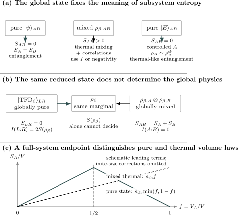
Three audits that prevent the most common confusion. The global-state ledger determines whether $S_A$ is pure-state entanglement or mixed-state entropy. A thermofield-double purification and an uncorrelated thermal product can have the same marginal $\rho_\beta$ while possessing different global entropy and mutual information. Finally, a mixed thermal volume law continues to $f=1$, whereas a globally pure state obeys complement symmetry and returns to zero. The curves show leading schematic terms; constraints, boundaries, and finite-size corrections remain model dependent.

Entropy of a Mixed Thermal State

The full Gibbs state

At finite temperature, a nontrivial Gibbs state is generally mixed:

$$\operatorname{Tr}\rho_\beta^2<1.$$

Its full-state entropy

$$\mathcal S_{AB}^{\mathrm{th}} = \mathcal S(\rho_{\beta,AB})$$

is thermodynamic entropy in dimensionless units. For a regular short-range system away from pathologies,

$$\mathcal S_{AB}^{\mathrm{th}} = s_{\mathrm{th}}(\beta)V +o(V),$$

where $s_{\mathrm{th}}$ is the dimensionless thermodynamic entropy density.

This full-state entropy is already enough to distinguish a thermal density operator from any pure eigenstate:

$$\mathcal S \left( \lvert E\rangle\langle E\rvert \right) = 0$$

at every finite size.

A reduced Gibbs state is not generally a local Gibbs state

Suppose a local Hamiltonian is decomposed as

$$H = H_A+H_B+H_{\partial},$$

where $H_{\partial}$ couples degrees of freedom across the boundary. The thermal marginal is

$$\rho_{\beta,A} = \operatorname{Tr}_B \left( \frac{e^{-\beta H}}{Z} \right).$$

In general,

$$\rho_{\beta,A} \ne \frac{e^{-\beta H_A}} {\operatorname{Tr}_A e^{-\beta H_A}}.$$

The obstruction is not merely that $H_A$ and $H_{\partial}$ fail to commute. Tracing out $B$ builds boundary correlations and interaction-dependent terms into the exact modular Hamiltonian

$$K_A := -\ln\rho_{\beta,A}.$$

Deep inside a large region of a short-range thermal phase, local observables may be well approximated by an appropriate bulk Gibbs description. The exact reduced operator still remembers the boundary and the environment.

Thermal volume law

For a large regular region $A$ in a homogeneous thermal phase,

$$\mathcal S(\rho_{\beta,A}) = s_{\mathrm{th}}(\beta)V_A +O(|\partial A|) +o(V_A),$$

with qualifications near critical points, for long-range interactions, in constrained sectors, and in continuum limits.

The leading term is present even if $A$ and $B$ are uncorrelated. It therefore cannot by itself measure entanglement across the boundary.

Infinite temperature is the cleanest counterexample

For a finite Hilbert space of dimension $d=d_Ad_B$, the $\beta=0$ Gibbs state is

$$\rho_0 = \frac{\mathbb I_{AB}}{d_Ad_B} = \frac{\mathbb I_A}{d_A} \otimes \frac{\mathbb I_B}{d_B}.$$

Its entropies are

$$\begin{aligned} \mathcal S_A &= \ln d_A, \\ \mathcal S_B &= \ln d_B, \\ \mathcal S_{AB} &= \ln(d_Ad_B). \end{aligned}$$

Yet

$$I(A:B)=0,$$

and the state is separable. On a lattice with local dimension $q$,

$$\mathcal S_A = V_A\ln q$$

is an exact volume law with no correlation at all. A volume law in a mixed thermal state is therefore not evidence of entanglement.

Mutual information cancels the bulk thermal term

For a bipartition of a finite volume,

$$V_A+V_B=V.$$

If the three entropies have regular leading thermal terms,

$$\begin{aligned} \mathcal S_A &= s_{\mathrm{th}}V_A +\delta_A, \\ \mathcal S_B &= s_{\mathrm{th}}V_B +\delta_B, \\ \mathcal S_{AB} &= s_{\mathrm{th}}V +\delta_{AB}, \end{aligned}$$

then

$$I(A:B) = \delta_A+\delta_B-\delta_{AB}.$$

The extensive bulk term cancels exactly. For short-range thermal systems, the remaining mutual information is often controlled by the interface and can obey an area law. It still counts total correlation, not entanglement alone.

Thermal entanglement can exist

Saying that thermal subsystem entropy is not an entanglement measure does not mean that every thermal state is separable. Interacting Gibbs states can remain entangled over a temperature range. The correct question is then whether $\rho_{\beta,AB}$ is entangled across $A\vert B$, which may be probed by:

• entanglement negativity;
• positive-partial-transpose tests where complete;
• entanglement witnesses;
• entanglement of formation or distillable entanglement in suitable settings.

The scalar $\mathcal S_A$ does not isolate that quantum component.

Entanglement Entropy of a Pure Many-Body State

Global purity and local mixedness

For a pure many-body wavefunction,

$$\rho_{AB} = \lvert\Psi\rangle\langle\Psi\rvert, \qquad \mathcal S_{AB}=0.$$

If $\rho_A$ is mixed, its mixedness cannot come from ensemble uncertainty in the total state. It comes from correlations with $B$, and

$$\mathcal S_A = \mathcal S_B$$

is the entanglement entropy.

Maximum possible value

For

$$d_A = \dim\mathcal H_A, \qquad d_B = \dim\mathcal H_B,$$

the Schmidt rank is at most $\min(d_A,d_B)$. Hence

$$\mathcal S_A \le \ln\min(d_A,d_B).$$

On a lattice of $q$-level sites,

$$\mathcal S_A \le \min(V_A,V_B)\ln q.$$

This bound already predicts a turnover at half-system size for any pure state.

Pure-state volume law

A family of pure states may satisfy

$$\mathcal S_A = s_{\mathrm{ent}}V_A +o(V_A)$$

when

$$V_A\ll V_B$$

or when $f<1/2$ is held fixed. This is genuine entanglement across $A\vert B$ because the total state is pure.

It cannot extend as a straight line through the entire range $0\le f\le1$. Complement symmetry requires

$$\mathcal S_A(f) = \mathcal S_A(1-f),$$

and

$$\mathcal S_A(1)=0.$$

A schematic thermalizing pure-state law is

$$\mathcal S_A \sim s_{\mathrm{ent}}V \min(f,1-f),$$

with model-dependent corrections. The corresponding mixed thermal entropy instead has leading behavior

$$\mathcal S_A^{\mathrm{th}} \sim s_{\mathrm{th}}Vf$$

and reaches the nonzero full thermal entropy at $f=1$.

The full-system endpoint test

Suppose numerical data show

$$\mathcal S_A \approx sV_A$$

for small regions. Before calling the coefficient thermal entropy, enlarge the region and ask:

Global state	Required endpoint
pure	$\mathcal S_A(V)=0$
mixed thermal	$\mathcal S_A(V)=s_{\mathrm{th}}V+o(V)$

This endpoint is more decisive than the word “volume law.”

Exact Comparison: Two Thermal Qubits and a Purification

One thermal qubit

Let

$$H = \epsilon\lvert1\rangle\langle1\rvert.$$

Its Gibbs state is

$$\rho_\beta = (1-r)\lvert0\rangle\langle0\rvert +r\lvert1\rangle\langle1\rvert,$$

where

$$r = \frac{e^{-\beta\epsilon}} {1+e^{-\beta\epsilon}}.$$

The dimensionless thermal entropy is the binary entropy

$$h_2(r) := -r\ln r -(1-r)\ln(1-r).$$

Uncorrelated thermal pair

Prepare two independent copies:

$$\rho_{AB}^{\mathrm{prod}} = \rho_{\beta,A} \otimes \rho_{\beta,B}.$$

Then

$$\begin{aligned} \mathcal S_A &= h_2(r), \\ \mathcal S_B &= h_2(r), \\ \mathcal S_{AB} &= 2h_2(r), \\ I(A:B) &= 0. \end{aligned}$$

Each subsystem has nonzero thermal entropy, but there is neither correlation nor entanglement between the qubits.

Pure thermal purification

Now define

$$\begin{aligned} \lvert\mathrm{TFD}_\beta\rangle_{LR} &= \sqrt{1-r}\, \lvert0\rangle_L\lvert0\rangle_R \\ &\quad + \sqrt r\, \lvert1\rangle_L\lvert1\rangle_R. \end{aligned}$$

The total state is pure:

$$\mathcal S_{LR}=0.$$

Tracing out either copy gives the same one-qubit Gibbs state:

$$\rho_L = \rho_R = \rho_\beta.$$

Therefore

$$\begin{aligned} \mathcal S_L &= \mathcal S_R = h_2(r), \\ I(L:R) &= 2h_2(r). \end{aligned}$$

The uncorrelated thermal pair and the pure purification have identical one-qubit marginals and identical one-qubit entropies. Their global entropy and correlations are completely different. Local entropy alone cannot choose between them.

Purification and the Exact Equality

General Gibbs purification

Let

$$H\lvert n\rangle = E_n\lvert n\rangle.$$

Introduce an auxiliary copy $R$ and define

$$\begin{aligned} \lvert\mathrm{TFD}_\beta\rangle_{LR} &= \frac{1}{\sqrt{Z(\beta)}} \sum_n e^{-\beta E_n/2} \\ &\quad\times \lvert n\rangle_L \lvert n\rangle_R. \end{aligned}$$

Then

$$\operatorname{Tr}_R \lvert\mathrm{TFD}_\beta\rangle \langle\mathrm{TFD}_\beta\rvert = \rho_{\beta,L}.$$

The Schmidt probabilities are

$$p_n = \frac{e^{-\beta E_n}}{Z},$$

so

$$\mathcal S_{\mathrm{ent}}(L:R) = -\sum_n p_n\ln p_n = \mathcal S(\rho_\beta).$$

Thus the dimensionless thermal entropy of $\rho_\beta$ equals the entanglement entropy between a system and a purifying copy in this pure state.

What the equality does and does not say

The equality is exact, but its labels matter:

Quantity	State	Partition
$\mathcal S_{\mathrm{th}}$	$\rho_{\beta,L}$	full physical system $L$
$\mathcal S_{\mathrm{ent}}$	$\lvert\mathrm{TFD}_\beta\rangle_{LR}$	$L\vert R$

It does not imply that the mixed Gibbs state is pure. It does not imply that its spatial entropy across a cut inside $L$ is entirely entanglement. It says that every mixed-state spectrum can be represented as Schmidt data of a larger pure state.

Different purifications are related by isometries on the purifying system. The auxiliary copy is therefore a representation choice unless a physical protocol identifies it with an actual second system.

Typical Pure States Can Look Thermal Locally

Haar-random benchmark

Consider a Haar-random pure state in

$$\mathcal H_A\otimes\mathcal H_B, \qquad d_A\le d_B.$$

The average purity of the smaller subsystem is

$$\mathbb E \operatorname{Tr}\rho_A^2 = \frac{d_A+d_B} {d_Ad_B+1}.$$

When $d_B\gg d_A$, this approaches $1/d_A$, the purity of the maximally mixed state.

The average von Neumann entropy is

$$\mathbb E\,\mathcal S_A = \sum_{k=d_B+1}^{d_Ad_B} \frac{1}{k} - \frac{d_A-1}{2d_B}.$$

For large $d_B$,

$$\mathbb E\,\mathcal S_A = \ln d_A - \frac{d_A}{2d_B} +\cdots.$$

If $d_A=q^{V_A}$, the leading term is

$$\mathcal S_A \approx V_A\ln q,$$

which is the infinite-temperature entropy density. The total random state remains pure.

Typical does not mean every Hamiltonian eigenstate

Haar-random vectors ignore:

• locality of the Hamiltonian;
• fixed energy density;
• particle-number or symmetry sectors;
• hydrodynamic slow modes;
• integrability and localization;
• the special structure of low-energy states.

The Page benchmark is an excellent null model for unconstrained Hilbert-space typicality. It is not a theorem that every highly excited eigenstate of every local Hamiltonian is Haar random.

Energy-shell typicality

Let $\mathcal H_R$ be a many-body energy shell with projector $P_R$ and dimension

$$d_R = \operatorname{Tr}P_R.$$

The normalized shell state is

$$\Omega_R = \frac{P_R}{d_R},$$

and its reduced state is

$$\Omega_A = \operatorname{Tr}_B\Omega_R.$$

Canonical typicality states, under precise finite-dimensional conditions, that for most pure vectors

$$\lvert\psi\rangle\in\mathcal H_R,$$

the reduced state

$$\rho_A^\psi = \operatorname{Tr}_B \lvert\psi\rangle\langle\psi\rvert$$

is close to $\Omega_A$ when the effective environment is sufficiently large.

If $A$ is weakly coupled to a large bath and the bath density of states varies smoothly over the relevant exchange energies, then

$$\Omega_A \approx \frac{e^{-\beta H_A}}{Z_A}.$$

The local state can therefore be approximately thermal even though

$$\mathcal S \left( \lvert\psi\rangle\langle\psi\rvert \right) = 0.$$

State closeness and entropy closeness

Define trace distance by

$$T(\rho,\sigma) := \frac12 \left\| \rho-\sigma \right\|_1.$$

For finite $d_A$ and suitable $T$,

$$\left| \mathcal S(\rho)-\mathcal S(\sigma) \right| \le T\ln(d_A-1) +h_2(T).$$

Thus trace-norm closeness implies entropy closeness for a fixed finite subsystem.

The factor $\ln d_A$ matters. If $A$ grows with the total system, $d_A$ grows exponentially. A trace-distance statement that is adequate for fixed $A$ may be too weak to control an extensive entropy. Extensive-subsystem claims require their own scaling analysis.

Pure Eigenstates and Subsystem Thermalization

Global eigenstate versus thermal ensemble

An exact energy eigenstate satisfies

$$H\lvert E_n\rangle = E_n\lvert E_n\rangle$$

and is pure:

$$\mathcal S \left( \lvert E_n\rangle\langle E_n\rvert \right) = 0.$$

An energy-matched microcanonical state,

$$\rho_{\mathrm{mc}}(E_n,\Delta E),$$

is mixed and generally has extensive thermodynamic entropy. These are different global density operators even if they predict nearly the same values for a selected class of observables.

Reduced-state form of ETH

For a subsystem $A$, define

$$\rho_A^{(n)} = \operatorname{Tr}_B \lvert E_n\rangle\langle E_n\rvert.$$

A strong subsystem form of the eigenstate thermalization hypothesis proposes, in suitable chaotic systems and limits,

$$\rho_A^{(n)} \approx \operatorname{Tr}_B \rho_{\mathrm{mc}}(E_n,\Delta E)$$

for subsystems small enough relative to the total system and after matching conserved charges.

Consequently,

$$\mathcal S \left( \rho_A^{(n)} \right) \approx \mathcal S \left( \rho_A^{\mathrm{mc}} \right).$$

For a large but sub-half-system region in a homogeneous phase, this can produce

$$\mathcal S_A^{(n)} = s_{\mathrm{th}}(e_n)V_A +\text{subleading terms}.$$

The left side is entanglement entropy because the eigenstate is pure. The right-side coefficient is thermodynamic because it is determined by an energy-matched ensemble. Agreement is a local reduced-state statement.

Fixed subsystem and finite subsystem fraction

Several limits must be distinguished.

For fixed $V_A$ while $V\to\infty$,

$$f = \frac{V_A}{V} \longrightarrow0.$$

This is the cleanest local-thermalization regime.

For a growing but subextensive subsystem,

$$V_A\to\infty, \qquad \frac{V_A}{V}\to0,$$

the subsystem can carry a thermodynamic entropy density while remaining a vanishing fraction of the whole.

For fixed

$$0<f<\frac12,$$

$A$ is extensive. Leading von Neumann entropy densities can still agree in chaotic systems, but reduced-state equality is a stronger and more delicate assertion. At and beyond half-system size, global purity is impossible to ignore.

Complement symmetry forces a Page-like turnover

For every pure eigenstate,

$$\mathcal S_A^{(n)} = \mathcal S_B^{(n)}.$$

If the leading thermal coefficient applies on the smaller side, the schematic finite-fraction form is

$$\mathcal S_A^{(n)} \sim s_{\mathrm{th}}(e_n) \min(V_A,V_B).$$

In terms of $f$,

$$\frac{\mathcal S_A^{(n)}}{V} \sim s_{\mathrm{th}}(e_n) \min(f,1-f).$$

This is a leading diagnostic, not a universal exact formula. Energy conservation, additional charges, boundaries, finite-size structure, and atypical eigenstates modify subleading terms and sometimes the leading behavior.

Rényi entropies are more sensitive

For

$$\alpha>0, \qquad \alpha\ne1,$$

the Rényi entropy is

$$\mathcal S_A^{(\alpha)} = \frac{1}{1-\alpha} \ln \operatorname{Tr}\rho_A^\alpha.$$

Rényi entropies weight the reduced-state spectrum differently from the von Neumann entropy. In an extensive subsystem of a chaotic eigenstate, Rényi entropy densities can depend nonlinearly on $f$ and need not equal the Rényi entropy density of the canonical mixed state at the same energy.

Therefore:

• matching the von Neumann entropy density does not prove equality of reduced spectra;
• matching local observables does not automatically fix all Rényi entropies;
• the limit $\alpha\to1$ and the thermodynamic limit require controlled ordering.

When thermal-like behavior fails

The thermal comparison is not universal. It can fail or require modification in:

• integrable systems with extensive conserved quantities;
• many-body localized regimes;
• quantum many-body scars and other atypical eigenstates;
• fragmented or kinetically constrained Hilbert spaces;
• symmetry-broken finite systems if sectors are mixed inconsistently;
• spectral-edge states and low-energy phases;
• systems with long-range interactions or unusual thermodynamic limits.

In integrable systems, a generalized Gibbs ensemble may replace the canonical one for selected local observables. In localized systems, excited eigenstates can obey an area law rather than the thermal volume law.

Unitary Dynamics and Thermal-Like Subsystems

Global entropy does not grow

For a closed system evolving unitarily,

$$\rho(t) = U(t)\rho(0)U^\dagger(t).$$

Unitary conjugation preserves the spectrum, so

$$\mathcal S(\rho(t)) = \mathcal S(\rho(0)).$$

If the initial state is pure,

$$\mathcal S_{AB}(t)=0$$

for all time.

Subsystem entropy can grow

The reduced state

$$\rho_A(t) = \operatorname{Tr}_B\rho(t)$$

does not evolve unitarily on $A$ alone. Interactions spread initially local information into correlations across the cut, allowing

$$\mathcal S_A(t)$$

to grow while the total entropy remains zero.

For a thermalizing quench, sufficiently small subsystems may approach energy-matched equilibrium reduced states:

$$\rho_A(t) \longrightarrow \rho_A^{\mathrm{eq}}$$

in an operational sense for the observables and time windows under study. Then

$$\mathcal S_A(t) \longrightarrow s_{\mathrm{eq}}V_A +\text{subleading terms}.$$

The late-time entropy is pure-state entanglement whose leading density can be thermodynamic.

Equilibration is not global convergence

The full pure state cannot converge in trace norm to a mixed Gibbs state under exact unitary evolution. Thermalization instead concerns:

• reduced states of restricted subsystems;
• expectation values of a selected observable algebra;
• time averages or typical late times;
• coarse-grained descriptions;
• limits in which recurrences are pushed to very long times.

This distinction separates entanglement growth from literal production of fine-grained global entropy.

Nonequilibrium Overview gives the operational trace-distance, diagonal-ensemble, timescale, and finite-size tests behind this local thermalization statement.

Other late-time ensembles

The equilibrium comparison depends on the dynamics:

System class	Candidate local stationary description
generic nonintegrable	microcanonical or canonical
integrable	generalized Gibbs ensemble
many-body localized	local-integral description; nonthermal
open system	stationary density operator of the channel

Calling every saturation value “the thermal entropy” erases these distinctions.

Four Different Volume Laws

The phrase “volume law” states a scaling form, not a physical mechanism.

State family	Global state	Leading small-region entropy	What the coefficient means
Gibbs state	mixed	$s_{\mathrm{th}}V_A$	local thermodynamic mixedness
Haar-random state	pure	$(\ln q)V_A$	near-maximal Hilbert-space entanglement
chaotic energy eigenstate	pure	$s_{\mathrm{th}}(e)V_A$ under ETH conditions	entanglement with thermal leading density
thermalizing post-quench state	pure	$s_{\mathrm{eq}}V_A$ at late times	dynamically generated entanglement

These laws can share a slope over a range of $V_A$ and still differ in:

• the full-system entropy;
• complement symmetry;
• the entanglement spectrum;
• Rényi entropies;
• conserved-charge blocks;
• mutual information;
• finite-size corrections;
• their response to changing ensemble or energy window.

Temperature Limits and Ground-State Cautions

Infinite temperature

At $\beta=0$, a finite unconstrained Hilbert space has

$$\rho_0 = \frac{\mathbb I}{d}, \qquad \mathcal S(\rho_0) = \ln d.$$

This is maximal thermal mixedness. A Haar-typical pure state’s small subsystem is nearly the same maximally mixed state, but the global pure-state entropy remains zero.

If a conserved sector is imposed, the infinite-temperature state within that sector is

$$\rho_{0,Q} = \frac{P_Q}{\operatorname{Tr}P_Q},$$

not the identity on the entire Hilbert space. Charge constraints can produce correlations and logarithmic finite-size corrections.

Zero temperature with a unique ground state

If the finite system has a unique ground state separated from excitations, then

$$\rho_\beta \longrightarrow \lvert0\rangle\langle0\rvert$$

as $\beta\to\infty$, and

$$\mathcal S(\rho_\beta) \longrightarrow0.$$

The ground state can nevertheless have nonzero spatial entanglement entropy:

$$\mathcal S_A = \mathcal S \left( \operatorname{Tr}_B \lvert0\rangle\langle0\rvert \right) >0.$$

Zero thermodynamic entropy does not imply a product ground state.

Degenerate ground spaces and order of limits

For an exactly $g$-fold degenerate ground space, the symmetric canonical limit may approach

$$\rho_{\beta\to\infty} = \frac{P_0}{g},$$

with

$$\mathcal S \left( \rho_{\beta\to\infty} \right) = \ln g.$$

A selected pure ground state instead has zero global entropy. In symmetry-breaking problems,

$$\lim_{h\to0} \lim_{V\to\infty}$$

can differ from

$$\lim_{V\to\infty} \lim_{h\to0}.$$

State preparation, symmetry sector, infinitesimal fields, and order of limits must be included in any residual-entropy or entanglement claim.

A Reliable Comparison Workflow

Step 1: name the density operator

Write the actual object:

$$\begin{gathered} \rho_\beta, \qquad \rho_{\mathrm{mc}}, \qquad \lvert E_n\rangle\langle E_n\rvert, \\ \rho_A, \qquad \overline\rho. \end{gathered}$$

Do not use the word “state” as a substitute for this choice.

Step 2: state the physical boundary

Specify whether the entropy belongs to:

• the entire isolated system;
• a spatial region;
• a mode or orbital subset;
• a system after tracing an environment;
• a doubled purification;
• a symmetry or energy shell.

Step 3: record purity before interpretation

Compute or establish

$$\operatorname{Tr}\rho^2.$$

For a bipartite total state, distinguish

$$\operatorname{Tr}\rho_{AB}^2$$

from

$$\operatorname{Tr}\rho_A^2.$$

A pure total state with a mixed marginal is the defining setting for entanglement entropy.

Step 4: match thermodynamic constraints

When comparing a pure eigenstate or quench to an ensemble, match at least:

• mean energy or energy density;
• particle number and other exact charges;
• symmetry sector;
• system size and boundary conditions;
• ensemble width;
• local Hamiltonian and couplings.

An energy-matched canonical state solves

$$\langle H\rangle_\beta = E.$$

At finite size, canonical and microcanonical reduced states need not agree exactly.

Step 5: compare more than one scalar

Useful checks include:

$$T \left( \rho_A, \rho_A^{\mathrm{th}} \right),$$

local expectation-value differences,

$$\Delta_O = \left| \operatorname{Tr} \left[ O_A \left( \rho_A-\rho_A^{\mathrm{th}} \right) \right] \right|,$$

mutual information, Rényi entropies, charge-sector probabilities, and the entanglement spectrum.

Equal von Neumann entropies do not imply equal density operators.

Step 6: vary subsystem fraction

Measure

$$\mathcal S_A(f)$$

for several $f$, including values on both sides of $1/2$ when possible. Check:

$$\mathcal S_A(f) \stackrel{?}{=} \mathcal S_A(1-f)$$

for a pure total state, and inspect the full-system endpoint.

Step 7: audit limits and errors

Report:

• the sequence of total sizes $V$;
• the region geometry and boundary area;
• whether $V_A$ is fixed, subextensive, or a fixed fraction;
• the order of $V\to\infty$, $\beta\to\infty$, and symmetry-breaking limits;
• truncation, sampling, and fitting errors;
• finite-size drift in entropy density and subleading terms.

Worked Diagnostic Checks

Check 1: same entropy, different global state

Suppose

$$\rho_A = \begin{pmatrix} 1-r & 0 \\ 0 & r \end{pmatrix}.$$

Knowing

$$\mathcal S_A = h_2(r)$$

does not determine whether $A$ belongs to a pure TFD state, an uncorrelated thermal product, a classically correlated mixture, or another purification. One must inspect $\rho_{AB}$ or additional correlations.

Check 2: pure-state endpoint

For a pure state on $V$ sites,

$$\mathcal S_A(V) = 0.$$

Any fitted law

$$\mathcal S_A = sV_A+b$$

that predicts a nonzero value at $V_A=V$ has been applied outside its regime. It may still describe $V_A\ll V$.

Check 3: zero mutual information at maximal thermal entropy

At $\beta=0$,

$$\rho_0 = \rho_{0,A}\otimes\rho_{0,B}.$$

Therefore

$$I(A:B) = 0$$

even though $\mathcal S_A$ and $\mathcal S_B$ are maximal. Local entropy and correlation are independent concepts.

Check 4: thermal coefficient from a pure eigenstate

If an eigenstate calculation gives

$$\frac{\mathcal S_A}{V_A} \longrightarrow s(e),$$

compare $s(e)$ with the microcanonical derivative

$$\frac{1}{T} = \left( \frac{\partial S_{\mathrm{th}}}{\partial E} \right)_{V,N}$$

or with an energy-matched canonical calculation. Agreement supports a thermal interpretation of the leading density. It does not change the exact identity

$$\mathcal S_{AB}=0.$$

Check 5: entropy agreement without state agreement

Two density operators can have the same entropy and different spectra. For a qutrit, many distinct probability triples

$$(p_1,p_2,p_3)$$

lie on the same constant-entropy contour. Therefore

$$\mathcal S(\rho_A) = \mathcal S(\sigma_A)$$

does not imply

$$\rho_A=\sigma_A.$$

Compare spectra, trace distance, relative entropy, or a sufficiently rich operator set.

Check 6: boundary term versus bulk term

If

$$\mathcal S_A = sV_A+a|\partial A|+\cdots,$$

then changing shape at fixed $V_A$ can change the boundary correction while preserving the bulk coefficient. A thermal entropy density should be extracted from a family of regions and sizes, not from one cut.

Common Mistakes

Calling every subsystem entropy entanglement

$\mathcal S_A$ is an entanglement measure only when the joint $AB$ state is pure. For mixed $\rho_{AB}$, it includes local uncertainty.

Calling every volume law thermal

Random pure states, Floquet states, post-quench states, and constrained sectors can have volume laws with different coefficients and corrections. State class and ensemble matching are required.

Forgetting the full-system entropy

A pure eigenstate has zero full-state entropy. An equilibrium mixed ensemble generally has extensive full-state entropy. Local agreement does not remove this distinction.

Treating a reduced Gibbs state as exactly local Gibbs

Boundary coupling and correlations generally make

$$\operatorname{Tr}_B e^{-\beta H}$$

different from a constant times $e^{-\beta H_A}$.

Confusing purification with physical duplication

A purification represents a mixed state using a larger pure state. The auxiliary system is not automatically a literal hidden copy of the laboratory.

Inferring state equality from entropy equality

Entropy is one spectral functional. Many density operators share the same value.

Applying ETH without its qualifiers

ETH is a hypothesis for suitable nonintegrable systems and observables. It is not a theorem for every eigenstate, Hamiltonian, subsystem fraction, or conserved sector.

Ignoring fixed charges

Particle number, magnetization, and other symmetries alter the reference ensemble, reduced-state block structure, and finite-size corrections.

Extending a small-region law past half the system

Pure-state complement symmetry forces a turnover. A linear thermal law for $f\ll1$ cannot be extrapolated to $f=1$.

Equating local equilibration with global mixing

Exact unitary evolution preserves the global spectrum. Local observables can thermalize while the full state remains pure.

Mixing dimensionless and thermodynamic units

Entanglement entropy is normally reported as $\mathcal S$ in nats or bits. Physical thermodynamic entropy is $k_{\mathrm B}\mathcal S$.

Hiding the order of limits

Zero temperature, infinite volume, vanishing symmetry-breaking field, long time, and large subsystem limits need not commute.

Exercises

1. Thermal marginal, two global completions

Let

$$\rho_\beta = \begin{pmatrix} 1-r & 0 \\ 0 & r \end{pmatrix}, \qquad 0<r<1.$$

Consider

$$\rho_{AB}^{(1)} = \rho_\beta\otimes\rho_\beta$$

and

$$\lvert\Psi\rangle_{AB} = \sqrt{1-r}\lvert00\rangle + \sqrt r\lvert11\rangle.$$

1. Show that both states have the same marginal on $A$.
2. Compute $\mathcal S_A$, $\mathcal S_{AB}$, $I(A:B)$, and $\mathcal S(A|B)$ for both global states.
3. Explain why $\mathcal S_A$ alone cannot identify entanglement.

Solution

For the product state,

$$\operatorname{Tr}_B \left( \rho_\beta\otimes\rho_\beta \right) = \rho_\beta \operatorname{Tr}\rho_\beta = \rho_\beta.$$

For the pure state,

$$\begin{aligned} \operatorname{Tr}_B \lvert\Psi\rangle\langle\Psi\rvert &= (1-r)\lvert0\rangle\langle0\rvert + r\lvert1\rangle\langle1\rvert \\ &= \rho_\beta. \end{aligned}$$

Thus both have

$$\mathcal S_A = h_2(r).$$

For the product state, additivity gives

$$\mathcal S_{AB}^{(1)} = 2h_2(r),$$

so

$$\begin{aligned} I^{(1)}(A:B) &= h_2(r)+h_2(r) \\ &\quad -2h_2(r) = 0. \end{aligned}$$

Its conditional entropy is

$$\mathcal S^{(1)}(A|B) = \mathcal S_{AB}^{(1)} -\mathcal S_B^{(1)} = h_2(r).$$

The second global state is pure, hence

$$\mathcal S_{AB}^{(2)}=0.$$

Its Schmidt probabilities are $1-r$ and $r$, so

$$\mathcal S_A^{(2)} = \mathcal S_B^{(2)} = h_2(r).$$

Therefore

$$I^{(2)}(A:B) = 2h_2(r)$$

and

$$\mathcal S^{(2)}(A|B) = -h_2(r).$$

The same $\mathcal S_A$ is local thermal mixedness in the product state and pure-state entanglement in the purification. The global entropy or correlation data are indispensable.

2. Infinite-temperature lattice

A chain of $V$ sites has local Hilbert-space dimension $q$ and no sector restriction. At infinite temperature:

1. Write the global density operator.
2. Find the entropy of a region containing $V_A$ sites.
3. Compute the mutual information between the region and its complement.
4. Decide whether the volume law is entanglement.

Solution

The full Hilbert-space dimension is

$$d=q^V.$$

At $\beta=0$,

$$\rho_0 = \frac{\mathbb I}{q^V}.$$

Because the identity factorizes across any site bipartition,

$$\rho_0 = \frac{\mathbb I_A}{q^{V_A}} \otimes \frac{\mathbb I_B}{q^{V-V_A}}.$$

Therefore

$$\mathcal S_A = \ln q^{V_A} = V_A\ln q,$$

and similarly

$$\mathcal S_B = (V-V_A)\ln q.$$

The full entropy is

$$\mathcal S_{AB} = V\ln q.$$

Hence

$$\begin{aligned} I(A:B) &= \mathcal S_A+\mathcal S_B-\mathcal S_{AB} \\ &= V_A\ln q + (V-V_A)\ln q \\ &\quad - V\ln q \\ &= 0. \end{aligned}$$

The entropy is exactly volume law, but the state is a product across the cut. The volume law is thermal mixedness, not entanglement.

3. General thermofield-double identity

For

$$\lvert\mathrm{TFD}_\beta\rangle = \frac{1}{\sqrt Z} \sum_n e^{-\beta E_n/2} \lvert n\rangle_L \lvert n\rangle_R,$$

prove:

$$\rho_L = \frac{e^{-\beta H_L}}{Z},$$

and

$$\mathcal S_L = \beta\langle H\rangle_\beta +\ln Z.$$

Why is the second expression both an entanglement entropy and a dimensionless thermal entropy?

Solution

Form the projector:

$$\begin{aligned} \rho_{LR}^{\mathrm{TFD}} &:= \lvert\mathrm{TFD}_\beta\rangle \langle\mathrm{TFD}_\beta\rvert, \\ \rho_{LR}^{\mathrm{TFD}} &= \frac{1}{Z} \sum_{m,n} e^{-\beta(E_m+E_n)/2} \\ &\quad\times \lvert m\rangle_L\langle n\rvert_L \\ &\quad\otimes \lvert m\rangle_R\langle n\rvert_R. \end{aligned}$$

Tracing $R$ uses

$$\operatorname{Tr}_R \left( \lvert m\rangle_R\langle n\rvert_R \right) = \delta_{mn}.$$

Thus

$$\begin{aligned} \rho_L &= \frac{1}{Z} \sum_n e^{-\beta E_n} \lvert n\rangle_L\langle n\rvert_L \\ &= \frac{e^{-\beta H_L}}{Z}. \end{aligned}$$

Since

$$\ln\rho_L = -\beta H_L-\ln Z,$$

its entropy is

$$\begin{aligned} \mathcal S_L &= -\operatorname{Tr} \left( \rho_L\ln\rho_L \right) \\ &= \beta\operatorname{Tr} \left( \rho_LH_L \right) +\ln Z \\ &= \beta\langle H\rangle_\beta +\ln Z. \end{aligned}$$

The joint $LR$ state is pure, so $\mathcal S_L$ is entanglement entropy across $L\vert R$. The marginal $\rho_L$ is a Gibbs state, so the same number is its dimensionless thermal entropy. The equality compares different state boundaries.

4. Pure-state system-fraction audit

Suppose a pure thermalizing state on volume $V$ has, for regions smaller than half the system,

$$\mathcal S_A \approx sV_A.$$

1. Extend the leading expression to all subsystem fractions using complement symmetry.
2. Evaluate it at $f=1/4$, $1/2$, $3/4$, and $1$.
3. Compare it with the mixed thermal law $\mathcal S_A^{\mathrm{th}}\approx sV_A$.

Solution

For a pure state,

$$\mathcal S_A = \mathcal S_B.$$

The smaller volume is

$$\min(V_A,V_B) = V\min(f,1-f).$$

The leading symmetric extension is therefore

$$\mathcal S_A^{\mathrm{pure}} \approx sV\min(f,1-f).$$

It gives

$$\begin{array}{c|c} f & \mathcal S_A^{\mathrm{pure}}/(sV) \\ \hline 1/4 & 1/4 \\ 1/2 & 1/2 \\ 3/4 & 1/4 \\ 1 & 0 \end{array}$$

The mixed thermal law gives

$$\frac{\mathcal S_A^{\mathrm{th}}}{sV} \approx f,$$

so its corresponding values are

$$\frac14, \quad \frac12, \quad \frac34, \quad 1.$$

The two agree on the smaller side in this schematic leading approximation, but differ beyond half-system size and at the full-system endpoint.

5. Cancellation of thermal bulk entropy

Assume

$$\begin{aligned} \mathcal S_A &= sV_A+a_A|\partial A|+c_A, \\ \mathcal S_B &= sV_B+a_B|\partial A|+c_B, \\ \mathcal S_{AB} &= s(V_A+V_B)+c_{AB}. \end{aligned}$$

Compute $I(A:B)$. What can and cannot be inferred if it scales with $|\partial A|$?

Solution

Substitution gives

$$\begin{aligned} I(A:B) &= \mathcal S_A+\mathcal S_B-\mathcal S_{AB} \\ &= sV_A+sV_B-s(V_A+V_B) \\ &\quad + (a_A+a_B)|\partial A| \\ &\quad + c_A+c_B-c_{AB}. \end{aligned}$$

The volume terms cancel:

$$\begin{aligned} I(A:B) &= (a_A+a_B)|\partial A| \\ &\quad + c_A+c_B-c_{AB}. \end{aligned}$$

An area-law mutual information is consistent with correlations localized near the interface in a short-range thermal phase. Mutual information counts total correlation, however. The area law alone does not separate classical correlation from quantum entanglement.

6. Entropy continuity for growing subsystems

Let

$$T \left( \rho_A,\sigma_A \right) = \varepsilon_V$$

and suppose $A$ contains $V_A$ sites of local dimension $q$.

1. Use the continuity bound to estimate the entropy difference.
2. What condition on $\varepsilon_V$ is sufficient for the entropy-density difference to vanish when $V_A\to\infty$?
3. Why does $\varepsilon_V\to0$ by itself not guarantee a small total entropy difference?

Solution

The subsystem dimension is

$$d_A=q^{V_A}.$$

The continuity estimate gives

$$\begin{aligned} & \left| \mathcal S(\rho_A) - \mathcal S(\sigma_A) \right| \\ &\quad \le \varepsilon_V \ln \left( q^{V_A}-1 \right) \\ &\qquad + h_2(\varepsilon_V). \end{aligned}$$

For large $V_A$,

$$\ln \left( q^{V_A}-1 \right) = V_A\ln q+o(1).$$

After dividing by $V_A$,

$$\begin{aligned} \frac{ \left| \mathcal S(\rho_A) - \mathcal S(\sigma_A) \right| }{V_A} &\le \varepsilon_V\ln q \\ &\quad + \frac{h_2(\varepsilon_V)}{V_A} +o(1). \end{aligned}$$

Thus $\varepsilon_V\to0$ is sufficient for the entropy-density difference to vanish.

The unnormalized entropy difference can still scale as

$$\varepsilon_V V_A\ln q.$$

For it to vanish, one needs a stronger condition such as

$$\varepsilon_VV_A\to0,$$

together with control of the binary-entropy term. This is why fixed-subsystem trace-distance results cannot be extrapolated casually to extensive entropies.

7. Zero temperature and degeneracy

A finite Hamiltonian has a $g$-fold exactly degenerate ground space with projector $P_0$.

1. Find the $\beta\to\infty$ canonical state if all ground states remain equally weighted.
2. Compute its global entropy.
3. Compare with a selected pure ground state.
4. Explain why neither answer alone determines the spatial entanglement entropy.

Solution

As $\beta\to\infty$, excited-state weights vanish and equal ground-state weights remain:

$$\rho_{\infty} = \frac{P_0}{g}.$$

Its $g$ nonzero eigenvalues are $1/g$, so

$$\mathcal S(\rho_\infty) = -g\frac1g\ln\frac1g = \ln g.$$

A selected normalized ground state

$$\lvert0,a\rangle$$

has density operator

$$\rho_a = \lvert0,a\rangle\langle0,a\rvert$$

and global entropy

$$\mathcal S(\rho_a)=0.$$

Spatial entanglement depends on the reduced state

$$\rho_{A,a} = \operatorname{Tr}_B\rho_a$$

or on the reduction of the mixed projector state. Either can have nonzero entropy, and different pure ground states or superpositions can have different entanglement. Global residual entropy does not determine spatial entanglement.

8. Entropy ledger after a global quench

A product state

$$\lvert\Psi(0)\rangle = \lvert\psi_A\rangle \otimes \lvert\psi_B\rangle$$

evolves under an interacting closed-system Hamiltonian.

1. Find $\mathcal S_{AB}(t)$.
2. State the relation between $\mathcal S_A(t)$ and $\mathcal S_B(t)$.
3. Explain how $\mathcal S_A(t)$ can approach an extensive thermal value without violating unitarity.
4. Name two situations in which the late-time coefficient need not be the canonical thermal entropy density.

Solution

The initial state is pure, and unitary evolution preserves purity:

$$\rho_{AB}(t) = U(t) \lvert\Psi(0)\rangle \langle\Psi(0)\rvert U^\dagger(t).$$

Therefore

$$\mathcal S_{AB}(t)=0$$

for every $t$.

Because the total state remains pure,

$$\mathcal S_A(t) = \mathcal S_B(t).$$

The interaction can entangle degrees of freedom across the cut. Information that was initially local becomes encoded in $A$–$B$ correlations, making $\rho_A(t)$ mixed even though $\rho_{AB}(t)$ is pure.

In a thermalizing regime and for a sufficiently small subsystem,

$$\rho_A(t) \approx \rho_A^{\mathrm{eq}}$$

at typical late times. Then

$$\mathcal S_A(t) \approx s_{\mathrm{eq}}V_A$$

can hold. This is entanglement entropy with a thermal leading density, not growth of global fine-grained entropy.

In an integrable system, conserved charges can lead to a generalized Gibbs description. In a many-body localized system, the state can fail to thermalize and exhibit much slower entanglement growth with a nonthermal saturation structure. Constrained systems and scarred dynamics provide further exceptions.

Summary

The von Neumann formula does not determine its own physical interpretation. The interpretation follows from a ledger:

$$\begin{gathered} \text{global density operator} \\ \Downarrow \\ \text{pure or mixed} \\ \Downarrow \\ \text{subsystem and discarded} \\ \text{degrees of freedom} \\ \Downarrow \\ \text{ensemble, constraints, and scaling limit}. \end{gathered}$$

For a globally pure bipartite state,

$$\mathcal S_{AB}=0, \qquad \mathcal S_A=\mathcal S_B,$$

and subsystem entropy is entanglement entropy. For a mixed thermal state, $\mathcal S_A$ includes ordinary thermal mixedness and is not a general entanglement measure. Mutual information removes independent bulk entropy but still counts both classical and quantum correlation.

A pure state can look thermal locally. Haar-typical vectors, energy-shell typicality, thermalizing eigenstates, and post-quench states provide distinct mechanisms by which

$$\rho_A \approx \rho_A^{\mathrm{th}}$$

and

$$\mathcal S_A \approx s_{\mathrm{th}}V_A$$

can emerge. The equality is local and limit dependent. Globally, the pure state still has zero entropy and obeys complement symmetry.

The decisive checks are global purity, mutual information, ensemble matching, subsystem fraction, the full-system endpoint, and sensitivity to Rényi index and conserved sectors. “Volume law” describes scaling; it does not by itself identify thermal entropy or entanglement.

References

1. H. Araki and E. H. Lieb, “Entropy Inequalities”, Communications in Mathematical Physics 18, 160–170 (1970).
2. W. Israel, “Thermo-Field Dynamics of Black Holes”, Physics Letters A 57, 107–110 (1976).
3. J. M. Deutsch, “Quantum Statistical Mechanics in a Closed System”, Physical Review A 43, 2046–2049 (1991).
4. D. N. Page, “Average Entropy of a Subsystem”, Physical Review Letters 71, 1291–1294 (1993).
5. S. K. Foong and S. Kanno, “Proof of Page’s Conjecture on the Average Entropy of a Subsystem”, Physical Review Letters 72, 1148–1151 (1994).
6. M. Srednicki, “Chaos and Quantum Thermalization”, Physical Review E 50, 888–901 (1994).
7. H. Tasaki, “From Quantum Dynamics to the Canonical Distribution: General Picture and a Rigorous Example”, Physical Review Letters 80, 1373–1376 (1998).
8. P. Calabrese and J. Cardy, “Evolution of Entanglement Entropy in One-Dimensional Systems”, Journal of Statistical Mechanics P04010 (2005).
9. S. Goldstein, J. L. Lebowitz, R. Tumulka, and N. Zanghì, “Canonical Typicality”, Physical Review Letters 96, 050403 (2006).
10. S. Popescu, A. J. Short, and A. Winter, “Entanglement and the Foundations of Statistical Mechanics”, Nature Physics 2, 754–758 (2006).
11. K. M. R. Audenaert, “A Sharp Continuity Estimate for the von Neumann Entropy”, Journal of Physics A 40, 8127–8136 (2007).
12. M. Rigol, V. Dunjko, and M. Olshanii, “Thermalization and Its Mechanism for Generic Isolated Quantum Systems”, Nature 452, 854–858 (2008).
13. M. M. Wolf, F. Verstraete, M. B. Hastings, and J. I. Cirac, “Area Laws in Quantum Systems: Mutual Information and Correlations”, Physical Review Letters 100, 070502 (2008).
14. P. Reimann, “Foundation of Statistical Mechanics under Experimentally Realistic Conditions”, Physical Review Letters 101, 190403 (2008).
15. A. M. Kaufman et al., “Quantum Thermalization through Entanglement in an Isolated Many-Body System”, Science 353, 794–800 (2016).
16. A. Dymarsky, N. Lashkari, and H. Liu, “Subsystem Eigenstate Thermalization Hypothesis”, Physical Review E 97, 012140 (2018).
17. J. R. Garrison and T. Grover, “Does a Single Eigenstate Encode the Full Hamiltonian?”, Physical Review X 8, 021026 (2018).
18. T.-C. Lu and T. Grover, “Rényi Entropy of Chaotic Eigenstates”, Physical Review E 99, 032111 (2019).

Cross-Links

• Volume Laws — Page typicality, finite-energy eigenstates, mixed thermal extensivity, and quench-generated plateaus.

• Mutual Information in Many-Body Systems — cancellation of independent thermal entropy, Gibbs-state bounds, and constrained-ensemble correlations.

• Many-Body Entanglement Overview — partition, state-class, information-measure, and scaling workflow.

• Entanglement Entropy in Many-Body Systems — spatial scaling, area and volume laws, continuum cautions, and numerical extraction.

• Area Laws — pure-state boundary scaling, thermal mutual-information bounds, and state-class caveats.

• Entropy in Quantum Statistical Mechanics — thermodynamic, ensemble, diagonal, and coarse-grained entropy.

• Thermal Density Operators — Gibbs states and equilibrium density operators.

• Microcanonical Ensemble — energy shells, widths, and microcanonical averages.

• Canonical Ensemble — canonical weights, partition functions, and energy matching.

• Ensemble Equivalence — thermodynamic conditions and finite-size limitations.

• Thermodynamic Limit — extensive quantities, boundary corrections, and order of limits.

• Subsystem Entropy — local mixedness in pure and mixed joint states.

• Purification — general purifications and their nonuniqueness.

• Entanglement Entropy — pure-state bipartite definition and Schmidt formula.

• Rényi Entropies — spectrum-sensitive entropy family.

• Mutual Information — total correlations in pure and mixed states.

• Proper and Improper Mixtures — operational and purification perspectives on mixed states.

• Entropy Production — open-system and thermodynamic entropy balances.

• Entanglement in Many-Body Physics — cross-volume orientation and applications.