Operator Entanglement and Scrambling Preview

Operator entanglement measures how nonseparably an operator acts across a chosen spatial cut. Scrambling asks whether initially local quantum information has become recoverable only from sufficiently nonlocal degrees of freedom. The two ideas are related, but they are not synonyms.

For a bipartite Hilbert space

$$\mathcal H = \mathcal H_A\otimes\mathcal H_B,$$

an operator can be treated as a vector in Hilbert–Schmidt space and decomposed as

$$\frac{O}{\lVert O\rVert_2} = \sum_{\alpha} s_\alpha\, A_\alpha\otimes B_\alpha, \qquad \sum_\alpha s_\alpha^2=1.$$

The operator entanglement entropy across $A|B$ is

$$S_{\mathrm{op}}(O;A|B) = -\sum_\alpha s_\alpha^2\ln s_\alpha^2.$$

This entropy answers a precise structural question: how many product operators are required across that cut? It does not, by itself, say how far the operator has spread, how much entanglement it creates from product states, whether the dynamics thermalizes, or whether a system is quantum chaotic.

In Heisenberg evolution,

$$W(t) = e^{iHt/\hbar} W e^{-iHt/\hbar},$$

an initially local operator can acquire support over an expanding region and become a superposition of many operator strings. An out-of-time-order correlator, or equivalently a suitable squared commutator, probes whether this evolved operator has become noncommuting with a distant local probe. A channel-state construction asks a stronger information-theoretic question: where can the input information be recovered from the output?

The practical hierarchy is

$$\begin{gathered} \text{operator support} \\[-2pt] \neq \\[-2pt] \text{operator entanglement}, \\[-2pt] \neq \\[-2pt] \text{state entanglement}, \\[6pt] \text{OTOC decay} \\[-2pt] \neq \\[-2pt] \text{scrambling without controls}, \\[-2pt] \neq \\[-2pt] \text{thermalization}. \end{gathered}$$

The point of this preview is to make those distinctions usable.

Canonical Scope

This page is the canonical home for the entanglement structure of operators in many-body quantum mechanics. It owns:

• Hilbert–Schmidt vectorization and its normalization conventions;
• the spatial operator Schmidt decomposition;
• operator Schmidt rank, spectrum, and entropies;
• the relation between operator entanglement and matrix-product-operator bond dimension;
• the distinction among operator entanglement, state entanglement, and entangling power;
• basic examples including product operators, CNOT, and SWAP;
• the entanglement-centered view of Heisenberg operator growth;
• a preview of squared commutators, OTOCs, butterfly fronts, and scrambling;
• the channel-state and tripartite-information viewpoint;
• the limited bridge to thermal quantum field theory and black-hole scrambling.

Neighboring pages retain separate canonical roles:

• Entanglement Entropy in Many-Body Systems owns spatial entanglement of states.
• Tensor Networks Preview owns tensor-network geometry and the broad relation between bond dimension and entanglement.
• Matrix Product States Preview owns MPS canonical forms, truncation, and state-focused one-dimensional algorithms.
• Channel-State Duality owns the Choi correspondence, marginal constraints, and channel reconstruction.
• Lieb–Robinson Bound owns the rigorous locality theorem and its assumptions.
• Semiclassical Quantum Chaos Preview owns the classical-to-quantum correspondence, periodic-orbit signatures, and semiclassical instability.
• Many-Body Quantum Chaos Preview owns symmetry-resolved spectral diagnostics, random-matrix universality windows, Thouless scales, and the relation to ETH.
• Time-Dependent Correlations owns ordinary time-ordered dynamical correlation functions.

Scrambling and OTOCs Preview owns detailed OTOC front analysis, thermal regularization choices, chaos-rate extraction, measurement protocols, and model-by-model scrambling phenomenology. Here those subjects are developed only far enough to explain what operator entanglement does and does not establish.

Assumptions and Convention Ledger

Unless stated otherwise:

• $\mathcal H=\mathcal H_A\otimes\mathcal H_B$ is finite dimensional;
• $A|B$ is a specified spatial tensor-factor cut;
• $\dim\mathcal H_A=d_A$, $\dim\mathcal H_B=d_B$, and $d=d_Ad_B$;
• logarithms are natural, so entropies are measured in nats;
• $H$ is time independent and evolution is unitary;
• $W$ and $V$ are bounded operators, often local unitaries or Pauli operators;
• thermal expectation values use

$$\rho_\beta = \frac{e^{-\beta H}}{Z}, \qquad Z = \operatorname{Tr}e^{-\beta H};$$

• operator entanglement uses the Hilbert–Schmidt inner product unless another convention is declared.

Gauge constraints, indistinguishable-particle subalgebras, continuum quantum fields, and nonunitary channels require additional factorization or regularization choices. Those choices are physical data, not notation that can be silently suppressed.

Two Hilbert–Schmidt normalizations are common:

$$\begin{aligned} \langle\!\langle X\vert Y\rangle\!\rangle_{\mathrm{HS}} &= \operatorname{Tr}(X^\dagger Y), \\ \langle\!\langle X\vert Y\rangle\!\rangle_{\infty} &= \frac{1}{d} \operatorname{Tr}(X^\dagger Y). \end{aligned}$$

The second is convenient at infinite temperature because every unitary has unit norm. This page uses the first convention for operator Schmidt decompositions and explicitly normalizes $O/\lVert O\rVert_2$. It uses the normalized-trace convention when expanding qubit operators in Pauli strings. Entropies agree once the operator vector has unit norm.

Operators as Vectors

Choose an orthonormal basis $\{\lvert i\rangle\}$ of $\mathcal H$. Column vectorization maps

$$O = \sum_{i,j} O_{ij} \lvert i\rangle\langle j\rvert$$

to

$$\lvert O\rangle\!\rangle = \sum_{i,j} O_{ij} \lvert i\rangle_{\mathrm{out}} \otimes \lvert j\rangle_{\mathrm{in}}.$$

The doubled vector satisfies

$$\langle\!\langle X\vert Y\rangle\!\rangle = \operatorname{Tr}(X^\dagger Y),$$

so

$$\lVert\lvert O\rangle\!\rangle\rVert^2 = \lVert O\rVert_2^2 = \operatorname{Tr}(O^\dagger O).$$

The normalized operator state is therefore

$$\lvert\widehat O\rangle\!\rangle = \frac{\lvert O\rangle\!\rangle} {\lVert O\rVert_2}.$$

Vectorization is an isometric bookkeeping map, not a claim that an arbitrary laboratory operator is literally a prepared pure state. It lets state-entanglement tools act on operator space.

Basis and transpose conventions

The identity

$$\lvert AOB^T\rangle\!\rangle = (A\otimes B) \lvert O\rangle\!\rangle$$

depends on the chosen vectorization convention. With a different ordering, the transpose or complex conjugation appears elsewhere. This basis dependence matters when reconstructing a channel from a Choi state.

For operator entanglement, a local basis change within $A$ or $B$ induces a local unitary transformation on the corresponding doubled operator space. It therefore leaves the operator Schmidt coefficients unchanged. A nonlocal redefinition of the cut does not.

Spatial Operator Schmidt Decomposition

Because

$$\mathcal L(\mathcal H) \cong \mathcal L(\mathcal H_A) \otimes \mathcal L(\mathcal H_B),$$

the normalized operator admits a Schmidt decomposition:

$$\frac{O}{\lVert O\rVert_2} = \sum_{\alpha=1}^{r_{\mathrm{op}}} s_\alpha\, A_\alpha\otimes B_\alpha.$$

The operator factors obey

$$\begin{aligned} \operatorname{Tr} \left( A_\alpha^\dagger A_\gamma \right) &= \delta_{\alpha\gamma}, \\ \operatorname{Tr} \left( B_\alpha^\dagger B_\gamma \right) &= \delta_{\alpha\gamma}, \end{aligned}$$

and

$$s_\alpha\geq0, \qquad \sum_\alpha s_\alpha^2=1.$$

The operator Schmidt rank satisfies

$$r_{\mathrm{op}} \leq \min(d_A^2,d_B^2).$$

It is one precisely when $O$ factorizes:

$$r_{\mathrm{op}}=1 \quad\Longleftrightarrow\quad O=O_A\otimes O_B$$

for a nonzero operator $O$.

Computing the spectrum

Choose Hilbert–Schmidt-orthonormal operator bases

$$\{E_\mu^A\}_{\mu=1}^{d_A^2}, \qquad \{E_\nu^B\}_{\nu=1}^{d_B^2},$$

and expand

$$\frac{O}{\lVert O\rVert_2} = \sum_{\mu,\nu} M_{\mu\nu} E_\mu^A\otimes E_\nu^B.$$

An ordinary singular-value decomposition,

$$M = U\,\operatorname{diag}(s_\alpha)\,V^\dagger,$$

produces the operator Schmidt coefficients. Equivalently, trace out the doubled $B$ degrees of freedom:

$$\rho_A^{\mathrm{op}} = \operatorname{Tr}_{B_{\mathrm{out}}B_{\mathrm{in}}} \left( \lvert\widehat O\rangle\!\rangle \langle\!\langle\widehat O\rvert \right).$$

Then

$$\operatorname{spec} \left( \rho_A^{\mathrm{op}} \right) = \{s_\alpha^2\}.$$

This is a reduced density operator in the auxiliary Hilbert–Schmidt construction. It should not be confused with the reduced physical state of a many-body wavefunction.

Operator Entropies

The von Neumann operator entanglement is

$$S_{\mathrm{op}} = -\operatorname{Tr} \left( \rho_A^{\mathrm{op}} \ln\rho_A^{\mathrm{op}} \right) = -\sum_\alpha s_\alpha^2\ln s_\alpha^2.$$

The Rényi operator entropies are

$$\begin{gathered} S_{\mathrm{op}}^{(n)} = \frac{1}{1-n} \ln \left( \sum_\alpha s_\alpha^{2n} \right), \\ n>0, \qquad n\neq1. \end{gathered}$$

Useful limits include

$$\begin{aligned} S_{\mathrm{op}}^{(0)} &= \ln r_{\mathrm{op}}, \\ S_{\mathrm{op}}^{(2)} &= -\ln \left( \sum_\alpha s_\alpha^4 \right), \\ S_{\mathrm{op}}^{(\infty)} &= -\ln \left( \max_\alpha s_\alpha^2 \right). \end{aligned}$$

The maximum possible entropy is

$$S_{\mathrm{op}} \leq \ln\min(d_A^2,d_B^2) = 2\ln\min(d_A,d_B).$$

Equality requires a flat operator Schmidt spectrum on the smaller operator space.

The linear operator entropy,

$$E_{\mathrm{op}}^{(2)} = 1- \operatorname{Tr} \left[ \left( \rho_A^{\mathrm{op}} \right)^2 \right] = 1-\sum_\alpha s_\alpha^4,$$

is common in analytic calculations because it is polynomial in the operator coefficients. Its numerical value is not the von Neumann entropy and should be labeled explicitly.

Matrix-Product-Operator Complexity

Across any cut of a one-dimensional matrix-product operator with bond dimension $\chi$,

$$r_{\mathrm{op}} \leq \chi,$$

and therefore

$$S_{\mathrm{op}} \leq \ln\chi.$$

An exact representation consequently requires

$$\chi \geq r_{\mathrm{op}} \geq e^{S_{\mathrm{op}}}.$$

For an approximate representation, order the Schmidt weights as

$$s_1^2 \geq s_2^2 \geq \cdots.$$

Keeping the largest $\chi$ terms produces a Hilbert–Schmidt truncation error

$$\epsilon_\chi^2 = \sum_{\alpha>\chi} s_\alpha^2.$$

The full spectrum, not the entropy alone, determines whether a modest $\chi$ gives an accurate approximation. Two operators can have the same $S_{\mathrm{op}}$ but very different discarded tails.

What the simulation statement does not say

Rapid operator-entanglement growth is a strong warning for global-fidelity MPO simulation. It is not a universal impossibility theorem for every computational task. Algorithms may exploit:

• conserved charges and block sparsity;
• integrability or free-particle structure;
• a restricted set of local observables;
• finite time or finite light-cone width;
• controlled dissipation or influence-functional compression;
• stochastic or quantum-computing methods that do not store the full operator.

Conversely, small entropy at one cut does not guarantee a cheap full simulation: every cut, every timestep, conditioning, and arithmetic cost still matter.

Three Different Entanglement Questions

State entanglement

For a physical state $\lvert\psi\rangle$,

$$S_A(\psi) = S \left( \operatorname{Tr}_B \lvert\psi\rangle\langle\psi\rvert \right)$$

depends on both the state and the spatial cut.

Operator entanglement

For a fixed operator $O$,

$$S_{\mathrm{op}}(O;A|B)$$

depends on the operator, the cut, and the Hilbert–Schmidt convention. No input state is required.

Entangling power

The entangling power of a unitary asks how much state entanglement it creates, on average, from product inputs:

$$e_p(U) = \int d\psi_A\,d\psi_B\, E \left[ U \left( \lvert\psi_A\rangle \otimes \lvert\psi_B\rangle \right) \right].$$

The value depends on the state ensemble and the chosen entanglement measure $E$. Operator entanglement and entangling power are related in some settings, but they are not equal.

Three Exact Examples

Product operator

If

$$O = O_A\otimes O_B,$$

then the normalized operator has one Schmidt coefficient,

$$s_1=1,$$

so

$$r_{\mathrm{op}}=1, \qquad S_{\mathrm{op}}=0.$$

A product operator may act nontrivially on every site. Large support therefore does not imply operator entanglement.

CNOT gate

Across the control–target cut,

$$U_{\mathrm{CNOT}} = P_0\otimes I + P_1\otimes X,$$

where

$$P_0 = \lvert0\rangle\langle0\rvert, \qquad P_1 = \lvert1\rangle\langle1\rvert.$$

The Hilbert–Schmidt-normalized factors

$$\left\{ P_0,P_1 \right\}, \qquad \left\{ \frac{I}{\sqrt2}, \frac{X}{\sqrt2} \right\}$$

are orthonormal. Since

$$\lVert U_{\mathrm{CNOT}}\rVert_2=2,$$

the normalized Schmidt decomposition is

$$\frac{U_{\mathrm{CNOT}}}{2} = \frac{1}{\sqrt2} P_0\otimes\frac{I}{\sqrt2} + \frac{1}{\sqrt2} P_1\otimes\frac{X}{\sqrt2}.$$

Thus

$$r_{\mathrm{op}}=2, \qquad S_{\mathrm{op}}=\ln2.$$

CNOT also has nonzero entangling power: for example,

$$U_{\mathrm{CNOT}} \left( \lvert+\rangle\otimes\lvert0\rangle \right) = \frac{ \lvert00\rangle+\lvert11\rangle }{\sqrt2}.$$

SWAP gate

For equal local dimensions $d$,

$$U_{\mathrm{SWAP}} = \sum_{i,j=1}^{d} \lvert i\rangle\langle j\rvert \otimes \lvert j\rangle\langle i\rvert.$$

The matrix units

$$E_{ij} = \lvert i\rangle\langle j\rvert$$

are Hilbert–Schmidt orthonormal. Because

$$\lVert U_{\mathrm{SWAP}}\rVert_2=d,$$

there are $d^2$ equal Schmidt coefficients:

$$s_{ij} = \frac{1}{d}.$$

Therefore

$$r_{\mathrm{op}} = d^2, \qquad S_{\mathrm{op}} = 2\ln d.$$

Yet

$$U_{\mathrm{SWAP}} \left( \lvert\psi\rangle_A \otimes \lvert\phi\rangle_B \right) = \lvert\phi\rangle_A \otimes \lvert\psi\rangle_B,$$

which is still a product state. SWAP has maximal operator entanglement across the cut but zero entangling power on product inputs. This is the cleanest counterexample to identifying the two quantities.

Heisenberg Operator Growth

Write

$$\operatorname{ad}_H(W) = [H,W].$$

The nested-commutator expansion is

$$W(t) = \sum_{n=0}^{\infty} \frac{1}{n!} \left( \frac{it}{\hbar} \right)^n \operatorname{ad}_H^n(W).$$

The first terms are

$$\begin{aligned} W(t) &= W + \frac{it}{\hbar} [H,W] \\ &\quad - \frac{t^2}{2\hbar^2} [H,[H,W]] + \cdots. \end{aligned}$$

For a local Hamiltonian

$$H = \sum_X h_X,$$

only terms $h_X$ whose support overlaps the current operator support contribute to the next commutator. Repeated commutators therefore grow support through connected interaction paths.

If $W$ begins on site $0$ and a probe $V_r$ lies graph distance $r$ away, the first nonzero term in

$$[W(t),V_r]$$

typically appears only after enough nested commutators have linked the two supports. This perturbative statement is the microscopic origin of an operator front; the Lieb–Robinson Bound turns locality into a nonperturbative norm estimate.

Pauli-String Expansion

For $N$ qubits, let

$$\mathcal P_N = \left\{ I,X,Y,Z \right\}^{\otimes N}.$$

Use the infinite-temperature inner product

$$(X,Y)_\infty = 2^{-N} \operatorname{Tr}(X^\dagger Y).$$

The Pauli strings are orthonormal:

$$(\mathcal S,\mathcal T)_\infty = \delta_{\mathcal S\mathcal T}.$$

An evolved operator has the expansion

$$W(t) = \sum_{\mathcal S\in\mathcal P_N} c_{\mathcal S}(t)\, \mathcal S,$$

with

$$c_{\mathcal S}(t) = 2^{-N} \operatorname{Tr} \left[ \mathcal S^\dagger W(t) \right].$$

If $W$ is unitary, Hilbert–Schmidt norm conservation gives

$$\sum_{\mathcal S} \left| c_{\mathcal S}(t) \right|^2 = 1.$$

Thus

$$p_{\mathcal S}(t) = \left| c_{\mathcal S}(t) \right|^2$$

is a normalized operator-weight distribution.

Site and endpoint weights

The nonidentity weight on site $j$ is

$$w_j(t) = \sum_{\mathcal S:\,\mathcal S_j\neq I} \left| c_{\mathcal S}(t) \right|^2.$$

A right-endpoint distribution can be defined by

$$p_R(j,t) = \sum_{\mathcal S:\,R(\mathcal S)=j} \left| c_{\mathcal S}(t) \right|^2,$$

where $R(\mathcal S)$ is the rightmost nonidentity site of the string. These weights track support growth. They do not determine the operator Schmidt spectrum.

Support is not operator entanglement

A single long string,

$$\mathcal S = \mathcal S_A\otimes\mathcal S_B,$$

has support on both sides but

$$S_{\mathrm{op}}(\mathcal S;A|B)=0.$$

Operator entanglement requires a nonseparable superposition of product strings:

$$W(t) = \sum_{\mu,\nu} M_{\mu\nu}(t) \mathcal S_\mu^A \otimes \mathcal S_\nu^B$$

with coefficient matrix $M(t)$ of rank greater than one.

This distinction is especially sharp in Clifford circuits. A Pauli operator evolves to another single Pauli string, so the individual operator can spread ballistically while retaining zero operator entanglement. Its distant commutators can nevertheless become large.

OTOC Preview

Let $W_x$ and $V_y$ be initially separated local unitaries. Define the thermal out-of-time-order correlator

$$\begin{aligned} \mathcal W_{xy}(t) &= W_x^\dagger(t) V_y^\dagger W_x(t) V_y, \\ F_{WV}(x-y,t) &= \operatorname{Tr} \left[ \rho_\beta\, \mathcal W_{xy}(t) \right]. \end{aligned}$$

The corresponding squared commutator is

$$\begin{aligned} K_{xy}(t) &= [W_x(t),V_y], \\ C_{WV}(x-y,t) &= \operatorname{Tr} \left[ \rho_\beta K_{xy}^\dagger(t) K_{xy}(t) \right]. \end{aligned}$$

For unitary $W_x$ and $V_y$,

$$C_{WV} = 2-2\operatorname{Re}F_{WV}.$$

The convention is important. Some authors define $C/2$, change the operator ordering, omit daggers for Hermitian operators, or normalize the correlator by disconnected thermal factors.

If the operators commute at $t=0$, then

$$\begin{aligned} F_{WV}(x-y,0) &= 1, \\ C_{WV}(x-y,0) &= 0. \end{aligned}$$

As the Heisenberg operator reaches $y$, the squared commutator can become nonzero. This makes $C(x,t)$ a state-weighted probe of operator–probe noncommutativity.

Exact Pauli-weight relation at infinite temperature

For a Hermitian unitary $W(t)$ expanded in Pauli strings, define

$$\begin{aligned} K_a(j,t) &= [W(t),\sigma_j^a], \\ C_a(j,t) &= 2^{-N} \operatorname{Tr} \left[ K_a^\dagger(j,t)K_a(j,t) \right], \\ a &\in \{x,y,z\}. \end{aligned}$$

A nonidentity single-site Pauli anticommutes with two of the three probe axes. Orthogonality of Pauli strings gives

$$\frac{1}{3} \sum_{a=x,y,z} C_a(j,t) = \frac{8}{3} w_j(t).$$

This exact identity explains why Pauli-averaged squared commutators image operator weight. It does not turn an OTOC into an operator-entanglement entropy.

Thermal Ordering and Regularization

At nonzero temperature, operator ordering around the thermal circle matters. A commonly used regularized correlator sets

$$y = \rho_\beta^{1/4}, \qquad y^4=\rho_\beta,$$

and defines

$$F_{\mathrm{reg}}(t) = \operatorname{Tr} \left[ yW^\dagger(t) yV^\dagger yW(t) yV \right].$$

This symmetric placement is not generally equal to the unregularized $F_{WV}$. In particular, the simple identity

$$C=2-2\operatorname{Re}F$$

belongs to the unregularized convention above and should not be transplanted without checking the inserted thermal factors.

Other choices include:

• the unregularized thermal OTOC;
• regulated contours with different imaginary-time separations;
• connected or normalized correlators;
• microcanonical or pure-state expectations;
• disorder, circuit, or operator-basis averages.

A reported exponent or scrambling time is meaningful only together with this convention ledger.

Operator Fronts

For local lattice Hamiltonians, a representative Lieb–Robinson estimate is

$$\begin{aligned} \left\lVert [W_x(t),V_y] \right\rVert &\leq C_0\, \lVert W_x\rVert \lVert V_y\rVert \\ &\quad\times \exp \left[ -\mu \left( r-v_{\mathrm{LR}}\lvert t\rvert \right) \right], \end{aligned}$$

where

$$r=d(x,y).$$

This is a state-independent operator-norm envelope. The number $v_{\mathrm{LR}}$ depends on the interaction assumptions and is usually not a measured propagation velocity.

A butterfly velocity $v_B$ is instead extracted from a chosen state-dependent diagnostic such as a contour

$$C(x,t)=C_\star.$$

If the contour is asymptotically ballistic,

$$x_\star(t) = v_Bt + o(t).$$

The butterfly front must remain compatible with an appropriate Lieb–Robinson envelope, but the numerical value of a convenient bound need not be close to $v_B$.

Front broadening

The front is generally not an infinitely sharp ray. In some one-dimensional random unitary circuits,

$$C(x,t) \approx \mathcal F \left( \frac{x-v_Bt} {\sqrt{4D_{\mathrm f}t}} \right),$$

so its width grows as

$$\Delta x_{\mathrm f}(t) \sim t^{1/2}.$$

This diffusive broadening is an exact or controlled result in particular circuit ensembles, not a universal law for every Hamiltonian. Integrability, conservation laws, long-range interactions, disorder, dimension, and the selected correlator can change the front shape.

Velocity-dependent growth

Outside a front, one sometimes writes a ray-dependent large-time form

$$C(vt,t) \sim \exp \left[ t\lambda(v) \right], \qquad v=\frac{x}{t}.$$

The front is associated schematically with

$$\lambda(v_B)=0.$$

This scaling form describes the small tail, not the saturated interior. A fitted $\lambda(v)$ is not automatically the thermal Lyapunov exponent $\lambda_L$ appearing in the chaos bound.

What Scrambling Means

Scrambling is the unitary delocalization of initially accessible quantum information into nonlocal correlations. After scrambling, the information has not been destroyed. Rather,

$$\begin{gathered} \text{small output subsystems contain} \\ \text{little recoverable information} \\ \text{about the input,} \\ \text{while a sufficiently large} \\ \text{joint subsystem can recover it}. \end{gathered}$$

This is stronger than saying that a local operator has broad support. It is also more specific than saying that a state has become highly entangled.

Scrambling is not erasure

For a closed system,

$$\rho(t) = U(t)\rho(0)U^\dagger(t)$$

preserves the global von Neumann entropy and distinguishability:

$$\begin{aligned} S[\rho(t)] &= S[\rho(0)], \\ D \left( U\rho U^\dagger, U\sigma U^\dagger \right) &= D(\rho,\sigma) \end{aligned}$$

for every unitarily invariant distinguishability measure $D$. Scrambling changes the subsystem accessibility of information.

Scrambling is not decoherence

Decoherence transfers information into an environment and can reduce system purity:

$$\operatorname{Tr}\rho_S^2 \longrightarrow \text{smaller}.$$

Ideal scrambling within a closed system can leave the global state pure. An OTOC signal may decay under either process, which is why experimental controls against imperfect reversal and noise are indispensable.

Scrambling is not thermalization

Thermalization concerns whether selected observables or subsystems approach predictions of an equilibrium ensemble. Scrambling concerns where information is encoded. They often accompany one another in chaotic many-body dynamics, but neither logically implies the other in complete generality.

Nonequilibrium Overview gives the canonical equilibration and ensemble-identification tests used in that distinction.

For example:

• integrable systems can spread operators without conventional thermalization;
• many-body-localized systems can develop slow dephasing and operator growth while retaining local memory;
• Clifford circuits can scramble some operator supports while remaining efficiently simulable;
• a system can locally equilibrate under constraints without approximating a Haar-random unitary channel.

Scrambling is not ordinary state entanglement growth

A quench may produce a state with increasing spatial entropy,

$$S_A(t),$$

while a scrambling diagnostic tracks an evolved operator or channel. The two growth processes can have different velocities:

$$v_E \neq v_B$$

in general, where $v_E$ denotes an entanglement-growth velocity and $v_B$ a butterfly velocity.

Diagnostic Comparison

Diagnostic	Object being analyzed	Primary inference
Support or Pauli weight	$W(t)$	where the operator has nontrivial action
Operator Schmidt spectrum	$W(t)$ or $U(t)$	spatial nonseparability and MPO complexity
Squared commutator	$W(t)$ and probe $V$	state-weighted noncommutativity
OTOC	four-point operator ordering	equivalent information to a declared squared commutator convention
State entropy	$\lvert\psi(t)\rangle$ or $\rho(t)$	correlations across a state partition
Choi mutual information	the channel state of $U$	input–output recoverability
Tripartite information	partitioned channel state	delocalization across output pieces
Spectral statistics	Hamiltonian or Floquet spectrum	symmetry-resolved spectral correlations

No single row licenses every inference in the others.

Channel-State Viewpoint

Let the physical input be

$$\mathcal H_{A_0}\otimes\mathcal H_{B_0},$$

and let a unitary map it to output systems $C$ and $D$:

$$U: \mathcal H_{A_0}\otimes\mathcal H_{B_0} \longrightarrow \mathcal H_C\otimes\mathcal H_D.$$

Introduce reference systems $A$ and $B$ with

$$\begin{aligned} \dim\mathcal H_A &= \dim\mathcal H_{A_0}, \\ \dim\mathcal H_B &= \dim\mathcal H_{B_0}. \end{aligned}$$

Prepare normalized maximally entangled pairs,

$$\begin{aligned} \lvert\Phi\rangle_{AA_0} &= \frac{1}{\sqrt{d_A}} \sum_{a=1}^{d_A} \lvert a\rangle_A \lvert a\rangle_{A_0}, \\ \lvert\Phi\rangle_{BB_0} &= \frac{1}{\sqrt{d_B}} \sum_{b=1}^{d_B} \lvert b\rangle_B \lvert b\rangle_{B_0}. \end{aligned}$$

The normalized channel state is

$$\begin{aligned} \lvert U\rangle\!\rangle_{ABCD} &= \left( I_{AB}\otimes U_{A_0B_0\to CD} \right) \\ &\quad\times \lvert\Phi\rangle_{AA_0} \lvert\Phi\rangle_{BB_0}. \end{aligned}$$

Up to tensor ordering and transpose conventions, this is the normalized vectorization of $U$.

The trivial input–output entanglement

For every unitary channel, the complete input reference $AB$ is maximally entangled with the complete output $CD$:

$$\rho_{AB} = \frac{I_{AB}}{d_Ad_B}.$$

Therefore

$$S(AB) = \ln(d_Ad_B).$$

This input–output entanglement is fixed by unitarity and does not diagnose scrambling. The informative question is how the input correlations are distributed among output pieces.

Spatial operator entanglement as a Choi cut

Suppose $C$ is the output associated with the left spatial region and $D$ with the right. Grouping doubled legs as

$$(A,C) \quad\big|\quad (B,D)$$

turns the channel state into the spatial operator cut. The entropy

$$S(AC)_{\lvert U\rangle\!\rangle}$$

is then the operator entanglement of $U$ across left and right, up to the declared leg-order convention.

Changing the Choi partition changes the physical question. The cut

$$AB|CD$$

tests input–output entanglement and is trivial for a unitary. The cut

$$AC|BD$$

tests spatial operator complexity. Mutual informations such as

$$I(A:C)$$

test whether a particular input subsystem remains locally accessible in a particular output subsystem.

Tripartite Information

For the channel state, define

$$I(A:C) = S(A)+S(C)-S(AC).$$

The tripartite information is

$$\begin{aligned} I_3(A:C:D) &= I(A:C) + I(A:D) \\ &\quad - I(A:CD). \end{aligned}$$

For a unitary channel state,

$$I(A:CD) = 2S(A) = 2\ln d_A.$$

If information about $A$ is nearly absent from $C$ and $D$ separately,

$$I(A:C) \approx 0, \qquad I(A:D) \approx 0,$$

but recoverable from $CD$ jointly, then

$$I_3(A:C:D) \approx -2\ln d_A.$$

Strongly negative tripartite information therefore captures a useful form of input–output delocalization.

Interpretation limits

Tripartite information is not a general entanglement measure and its sign is not a universal if-and-only-if test for every notion of chaos. Its interpretation depends on:

• which input and output subsystems are chosen;
• subsystem dimensions;
• von Neumann versus Rényi definitions;
• whether the map is unitary, noisy, postselected, or averaged;
• finite-size and conservation-law constraints;
• whether recovery is assessed exactly or approximately.

For a nonunitary channel, information can genuinely leak to an environment. Negative $I_3$ within the observed output then need not mean that the information remains globally recoverable there.

Relation Between OTOCs and Channel Information

The OTOC and Choi viewpoints are connected by operator-basis averaging. After fixing:

• complete orthonormal operator bases on selected input and output subsystems;
• a normalized-trace convention;
• a Rényi-2 entropy convention;
• the input–output leg ordering;

a basis-averaged family of OTOCs can be rewritten in terms of Rényi mutual information in the unitary channel state.

Schematically,

$$\begin{gathered} \text{average over input} \\ \text{and output operators} \\ \longleftrightarrow \\ \text{Rényi-2 input–output} \\ \text{mutual information}. \end{gathered}$$

Decay of a sufficiently complete OTOC family then indicates that an input operator is no longer correlated with a small output region. A single specially chosen OTOC is not the same data as the complete average.

Likewise,

$$-I_3$$

summarizes channel-wide delocalization, whereas

$$C_{WV}(x,t)$$

tests one evolved operator against one probe in one state or ensemble.

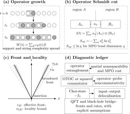
Four distinct layers of information spreading. (a) Local dynamics expands operator support and string complexity. (b) The operator Schmidt coefficients $s_\alpha$ determine operator entanglement and constrain matrix-product-operator bond dimension $\chi$. (c) A state-dependent butterfly front with velocity $v_B$ lies within an appropriate Lieb–Robinson locality envelope; front broadening is model dependent. (d) Operator entropy, OTOCs, and Choi-state tripartite information support different inferences. Quantum-field-theory and black-hole connections require additional thermal, large-system, and analyticity assumptions.

Operator Entanglement of the Evolution Operator

The full time-evolution operator,

$$U(t) = e^{-iHt/\hbar},$$

is initially a product across every spatial cut:

$$U(0) = I_A\otimes I_B.$$

Thus

$$S_{\mathrm{op}}[U(0)]=0.$$

Interactions crossing a cut can increase the operator Schmidt rank. In a local circuit of depth $n$, only gates whose causal cones cross the cut can contribute to the cut entropy. Consequently, locality gives finite-rate bounds on operator-entanglement production.

The operator entanglement of $U(t)$ and that of a local $W(t)$ are different quantities:

$$S_{\mathrm{op}}[U(t)] \neq S_{\mathrm{op}}[W(t)]$$

in general. The first measures the spatial complexity of the complete propagator. The second measures the complexity of one Heisenberg-evolved observable.

Growth laws are model dependent

Examples found in controlled models include:

• linear growth followed by volume-law saturation in chaotic Floquet systems;
• slower, sometimes logarithmic, growth in localized regimes;
• algebraic or otherwise structured growth in integrable systems;
• bounded growth for special conserved or solitonic operators;
• exactly tractable growth in free, Clifford, and dual-unitary circuits.

These are families of behavior, not a binary theorem that “linear means chaotic” and “logarithmic means integrable.”

Black-Hole and Quantum-Field-Theory Bridge

The modern scrambling language connects lattice many-body physics, quantum information, thermal quantum field theory, and holography through a common question: how does a small perturbation become difficult to recover from simple observables?

Holographic shock waves

In a two-sided anti-de Sitter black-hole geometry, an early infalling perturbation is exponentially blueshifted relative to a later probe. In the bulk description it produces a near-horizon shock wave. In the boundary field theory, the corresponding time ordering appears in an OTOC.

The bridge is qualitative and quantitative in controlled holographic regimes:

$$\begin{gathered} \text{early perturbation} \longleftrightarrow \text{shock wave}, \\ \text{shock wave} \longleftrightarrow \text{OTOC deviation}. \end{gathered}$$

This does not mean every many-body OTOC literally describes a black hole. Holographic calculations involve special large-$N$, strongly coupled quantum field theories and a semiclassical gravitational limit.

Thermal exponential window

In a suitable large-system thermal regime, a regularized OTOC may have an intermediate-time form

$$\frac{F_{\mathrm{reg}}(t)} {F_{\mathrm d}} \approx 1 - \varepsilon e^{\lambda_L t},$$

where:

• $F_{\mathrm d}$ is an appropriate disconnected scale;
• $\varepsilon$ is small in a controlled large-system expansion;
• $\lambda_L$ is a thermal many-body Lyapunov exponent;
• the approximation holds after local dissipation but before saturation.

The corresponding scrambling time estimate is

$$t_\ast \sim \frac{1}{\lambda_L} \ln\frac{1}{\varepsilon}.$$

Not every OTOC has such a clean window. Finite local Hilbert spaces, front broadening, conservation laws, integrability, operator selection, and small system size can obscure or eliminate it.

The thermal chaos bound

Under analyticity, boundedness, factorization, and timescale-separation assumptions, the thermal growth rate obeys

$$\lambda_L \leq \frac{2\pi k_{\mathrm B}T}{\hbar} = \frac{2\pi}{\beta\hbar}.$$

The bound applies to the relevant regularized thermal OTOC regime. It is not:

• a bound on every fitted front exponent $\lambda(v)$;
• a bound on classical Lyapunov exponents in arbitrary systems;
• a claim that every chaotic quantum model saturates it;
• a definition of quantum chaos;
• a theorem that any rapid OTOC decay is caused by scrambling.

Some semiclassical holographic black holes saturate the bound at leading order. Calling them “maximally chaotic” refers to this specific rate under these assumptions, not to every conceivable measure of complexity or randomness.

Relativistic and lattice causal structure

Relativistic quantum field theory has a microscopic causal speed:

$$[W(x,t),V(0,0)] = 0$$

at spacelike separation for local observables in an ideal continuum theory. A thermal butterfly front can propagate within that causal cone.

Local lattice systems instead have an emergent Lieb–Robinson envelope. The analogy is

$$\begin{gathered} \text{relativistic QFT:} \\ \text{light cone and thermal butterfly front}; \\[4pt] \text{local lattice system:} \\ \text{Lieb–Robinson envelope} \\ \text{and OTOC or commutator front}. \end{gathered}$$

The analogy should not erase their different ultraviolet structures.

Fast Scrambling

Suppose

$$\varepsilon \sim \frac{1}{N_{\mathrm{eff}}}.$$

Then an exponential OTOC window gives

$$t_\ast \sim \frac{1}{\lambda_L} \ln N_{\mathrm{eff}}.$$

If the chaos bound is saturated,

$$t_\ast \sim \frac{\beta\hbar}{2\pi} \ln N_{\mathrm{eff}}.$$

This logarithmic scaling motivates the fast-scrambler language for all-to-all systems and black holes. In black-hole applications, the effective size is often expressed through an entropy scale, giving schematically

$$t_\ast \sim \frac{\beta\hbar}{2\pi} \ln S_{\mathrm{BH}}.$$

Locality changes the question

In a $D$-dimensional local system of linear size $L$, information cannot influence the entire sample before a propagation time of order

$$t_{\mathrm{travel}} \gtrsim \frac{L}{v_B}.$$

A local system can have rapid local operator growth and still require a system-size-dependent travel time for global scrambling. One should not compare an all-to-all logarithmic estimate with a local lattice time without identifying geometry, connectivity, and the information-recovery task.

Experimental Access

Echo protocols

Many OTOC protocols require:

1. forward evolution under $H$;
2. insertion of a local perturbation;
3. approximate backward evolution under $-H$;
4. a final overlap or observable measurement.

Imperfect reversal can mimic OTOC decay. A convincing experiment therefore measures independent fidelity or purity controls and varies the perturbation, evolution time, and reversal calibration.

Interferometric and two-copy protocols

Ancilla interferometry and two-copy measurements can access operator orderings without reconstructing the full state. Their resource requirements and noise channels differ from echo protocols.

Teleportation verification

Scrambling-assisted teleportation protocols combine an OTOC-like success probability with a conditional teleportation fidelity. The fidelity helps distinguish coherent scrambling from ordinary decoherence: noise may reduce the OTOC signal without enabling faithful recovery.

What has been demonstrated

Controlled experiments have measured OTOC-related quantities in nuclear-magnetic-resonance processors, trapped-ion simulators, and programmable quantum circuits. These are important demonstrations of protocols and finite-system information spreading. They are not, by themselves, evidence that the device realizes a thermodynamic-limit chaos exponent or a black-hole regime.

Numerical Workflow

A reproducible operator-entanglement and scrambling study should record the following ledger.

Define the object and cut

Specify whether the calculation concerns:

$$\begin{gathered} U(t), \qquad W(t), \\ \text{a channel or a density operator}. \end{gathered}$$

Specify the tensor-factor cut and any symmetry or gauge-sector convention.

Normalize

Report whether the inner product is

$$\operatorname{Tr}(X^\dagger Y)$$

or

$$d^{-1}\operatorname{Tr}(X^\dagger Y).$$

Verify

$$\sum_\alpha s_\alpha^2=1.$$

Resolve the full Schmidt tail

Report:

$$r_{\mathrm{op}}, \qquad S_{\mathrm{op}}, \qquad S_{\mathrm{op}}^{(2)}, \qquad \epsilon_\chi^2.$$

Entropy without discarded weight is not enough to assess an MPO approximation.

Map the front

Compute $C(x,t)$ for several separations and extract $v_B$ from more than one contour $C_\star$. Test sensitivity to:

• the time window;
• the contour value;
• boundary reflections;
• system size;
• operator choice;
• temperature or energy density;
• front-broadening ansatz.

Keep rate and velocity distinct

Report separately:

$$v_B, \qquad \Delta x_{\mathrm f}(t), \qquad \lambda(v), \qquad \lambda_L.$$

Do not infer one from another without a model-specific derivation.

Control false positives

Compare with:

• an integrable or noninteracting limit;
• symmetry-resolved dynamics;
• a no-perturbation echo;
• purity or Loschmidt-fidelity diagnostics;
• bond-dimension and timestep convergence;
• alternate local probes;
• exact diagonalization at smaller size.

Add a recovery diagnostic when claiming scrambling

For a channel-level claim, compute input–output mutual information, tripartite information, decoupling error, or a verified teleportation fidelity. This strengthens an inference beyond a single decaying correlator.

Worked Diagnostic Examples

A long Pauli string

Consider

$$W = X_1Z_2Z_3\cdots Z_{N-1}X_N.$$

Across any spatial cut,

$$W = W_A\otimes W_B.$$

Therefore

$$S_{\mathrm{op}}(W)=0.$$

Nevertheless, for a site $j$ on which $W$ has a $Z$ factor,

$$[W,X_j]\neq0.$$

An OTOC with $X_j$ can therefore indicate nontrivial support while operator entanglement remains zero.

A sum of two strings

Let

$$O = \frac{1}{\sqrt2} \left( X_A\otimes X_B + Z_A\otimes Z_B \right),$$

where all four factors are Hilbert–Schmidt normalized and the two operators on each side are orthogonal. The Schmidt coefficients are

$$s_1=s_2=\frac{1}{\sqrt2},$$

so

$$S_{\mathrm{op}}(O)=\ln2.$$

The nonseparable sum, not merely two-sided support, creates operator entanglement.

Idealized channel delocalization

Suppose an input subsystem $A$ has dimension $q$ and, in a unitary channel state,

$$I(A:C) \approx I(A:D) \approx 0.$$

Because

$$I(A:CD)=2\ln q,$$

one finds

$$I_3(A:C:D) \approx -2\ln q.$$

The input is inaccessible from either output piece alone but remains encoded in their union.

Common Mistakes

• Calling the entanglement of a physical state “operator entanglement.”
• Omitting the operator normalization before interpreting $s_\alpha^2$ as probabilities.
• Forgetting that the operator Schmidt spectrum depends on the chosen spatial cut.
• Treating vectorization as basis independent without tracking transpose conventions.
• Equating operator Schmidt rank with spatial support size.
• Assuming a large operator entropy implies large entangling power; SWAP disproves this.
• Assuming broad support implies nonzero operator entropy; a single long product string disproves this.
• Using $S_{\mathrm{op}}\leq\ln\chi$ as if entropy alone determined truncation error.
• Comparing OTOCs that use different thermal contours or normalizations.
• Using $C=2-2\operatorname{Re}F$ for a regularized thermal OTOC without rederiving it.
• Calling every early exponential fit a Lyapunov exponent.
• Identifying the butterfly velocity with a Lieb–Robinson velocity.
• Ignoring front broadening when fitting $v_B$.
• Interpreting one decaying OTOC as complete evidence of scrambling.
• Failing to distinguish coherent scrambling from imperfect time reversal or decoherence.
• Treating negative tripartite information as a universal chaos theorem.
• Applying the thermal chaos bound outside its analytic and timescale assumptions.
• Using black-hole language for a finite circuit without stating the limited analogy.

Exercises

Exercise 1: Vectorization isometry

Using

$$\lvert X\rangle\!\rangle = \sum_{i,j} X_{ij} \lvert i\rangle\otimes\lvert j\rangle,$$

show that

$$\langle\!\langle X\vert Y\rangle\!\rangle = \operatorname{Tr}(X^\dagger Y).$$

Solution

Directly,

$$\begin{aligned} \langle\!\langle X\vert Y\rangle\!\rangle &= \sum_{i,j,k,l} X_{ij}^\ast Y_{kl} \langle i\vert k\rangle \langle j\vert l\rangle \\ &= \sum_{i,j} X_{ij}^\ast Y_{ij}. \end{aligned}$$

Meanwhile,

$$\operatorname{Tr}(X^\dagger Y) = \sum_j (X^\dagger Y)_{jj} = \sum_{i,j} X_{ij}^\ast Y_{ij}.$$

The two expressions agree.

Exercise 2: Maximum operator entropy

Prove that

$$S_{\mathrm{op}} \leq \ln\min(d_A^2,d_B^2).$$

When is equality possible?

Solution

The coefficient matrix of the operator expansion has at most

$$r_{\max} = \min(d_A^2,d_B^2)$$

nonzero singular values. The Shannon entropy of the probabilities

$$p_\alpha=s_\alpha^2$$

is maximized, for fixed support size $r_{\max}$, by the uniform distribution:

$$p_\alpha = \frac{1}{r_{\max}}.$$

Therefore

$$S_{\mathrm{op}} \leq -r_{\max} \frac{1}{r_{\max}} \ln\frac{1}{r_{\max}} = \ln r_{\max}.$$

Equality is possible when the operator has full Schmidt rank on the smaller operator space and all nonzero Schmidt weights are equal.

Exercise 3: CNOT spectrum

Use

$$U_{\mathrm{CNOT}} = P_0\otimes I + P_1\otimes X$$

to derive its operator Schmidt coefficients and entropy.

Solution

The control operators satisfy

$$\operatorname{Tr}(P_aP_b) = \delta_{ab}.$$

On the target,

$$\operatorname{Tr} \left[ \left( \frac{I}{\sqrt2} \right)^\dagger \frac{X}{\sqrt2} \right] = 0,$$

and both $I/\sqrt2$ and $X/\sqrt2$ have unit Hilbert–Schmidt norm. Hence

$$U_{\mathrm{CNOT}} = \sqrt2 P_0\otimes\frac{I}{\sqrt2} + \sqrt2 P_1\otimes\frac{X}{\sqrt2}.$$

Since $\lVert U_{\mathrm{CNOT}}\rVert_2=2$, normalization gives

$$s_1=s_2=\frac{1}{\sqrt2}.$$

Thus

$$S_{\mathrm{op}} = -2 \left( \frac12\ln\frac12 \right) = \ln2.$$

Exercise 4: SWAP versus entangling power

Show that the $d$-dimensional SWAP gate has

$$S_{\mathrm{op}}=2\ln d$$

but maps every product state to a product state.

Solution

Write

$$U_{\mathrm{SWAP}} = \sum_{i,j} E_{ij}\otimes E_{ji}.$$

There are $d^2$ Hilbert–Schmidt-orthonormal terms. The unitary norm is

$$\lVert U_{\mathrm{SWAP}}\rVert_2 = \sqrt{\operatorname{Tr}I_{d^2}} = d.$$

Therefore every normalized Schmidt coefficient is $1/d$, and

$$S_{\mathrm{op}} = -d^2 \frac{1}{d^2} \ln\frac{1}{d^2} = 2\ln d.$$

For arbitrary local states,

$$U_{\mathrm{SWAP}} \lvert\psi\rangle_A \lvert\phi\rangle_B = \lvert\phi\rangle_A \lvert\psi\rangle_B.$$

The output remains a product, so every product-input entanglement measure vanishes. Hence the product-state entangling power is zero.

Exercise 5: Locality from nested commutators

Consider a nearest-neighbor chain

$$H = \sum_j h_{j,j+1}.$$

If $W_0$ is supported only on site $0$, show that

$$\operatorname{ad}_H^n(W_0)$$

is supported no farther than $n$ bonds from site $0$. Conclude that a probe $V_r$ at distance $r$ has no contribution to

$$[W_0(t),V_r]$$

through order $t^{r-1}$.

Solution

For $n=0$, the support is site $0$. Suppose the support after $n$ nested commutators lies within distance $n$. A term

$$[h_{j,j+1},O]$$

vanishes unless the bond $\{j,j+1\}$ overlaps the support of $O$. A nonzero commutator can therefore enlarge the support by at most one neighboring site. By induction,

$$\operatorname{supp} \left[ \operatorname{ad}_H^n(W_0) \right] \subseteq \{j:d(j,0)\leq n\}.$$

If $n<r$, that support is disjoint from $V_r$, so

$$\left[ \operatorname{ad}_H^n(W_0), V_r \right] = 0.$$

The series for $[W_0(t),V_r]$ therefore begins no earlier than order $t^r$. This perturbative order is consistent with, but weaker than, a Lieb–Robinson bound.

Exercise 6: OTOC–commutator identity

For unitary $W$ and $V$, prove

$$\begin{aligned} \left\langle [W,V]^\dagger[W,V] \right\rangle &= 2 \\ &\quad - 2\operatorname{Re} \left\langle W^\dagger V^\dagger WV \right\rangle. \end{aligned}$$

Solution

Expand:

$$\begin{aligned} [W,V]^\dagger[W,V] &= V^\dagger W^\dagger WV \\ &\quad - V^\dagger W^\dagger VW \\ &\quad - W^\dagger V^\dagger WV \\ &\quad + W^\dagger V^\dagger VW. \end{aligned}$$

Unitarity reduces the first and last terms to $I$. The two middle expectation values are complex conjugates of one another, using cyclicity of the trace for a density-operator expectation. Therefore

$$\begin{aligned} \left\langle [W,V]^\dagger[W,V] \right\rangle &= 2-F-F^\ast \\ &= 2-2\operatorname{Re}F. \end{aligned}$$

Exercise 7: Pauli-averaged site weight

Let $W(t)$ be a Hermitian unitary expanded in Pauli strings. Show that

$$\frac13 \sum_{a=x,y,z} C_a(j,t) = \frac83w_j(t).$$

Solution

For a Pauli string $\mathcal S$, the local factor $\mathcal S_j$ is either $I$ or one of $X,Y,Z$.

If

$$\mathcal S_j=I,$$

then $\mathcal S$ commutes with all three probes and contributes zero.

If

$$\mathcal S_j\in\{X,Y,Z\},$$

then it commutes with one probe axis and anticommutes with the other two. For an anticommuting pair,

$$[\mathcal S,\sigma_j^a] = 2\mathcal S\sigma_j^a,$$

whose normalized squared Hilbert–Schmidt norm is $4$. Averaging over the three axes gives

$$\frac{0+4+4}{3} = \frac83.$$

Pauli orthogonality removes cross terms between distinct strings, so summing their probabilities produces

$$\begin{aligned} \frac13\sum_a C_a(j,t) &= \frac83 \sum_{\substack{\mathcal S:\\\mathcal S_j\neq I}} \lvert c_{\mathcal S}(t)\rvert^2 \\ &= \frac83w_j(t). \end{aligned}$$

Exercise 8: Ideal channel scrambling

In a unitary channel state, let $\dim A=q$ and suppose

$$I(A:C)=I(A:D)=0.$$

Find $I_3(A:C:D)$ and explain why the result describes delocalization rather than information loss.

Solution

For a unitary channel state,

$$I(A:CD) = 2S(A) = 2\ln q.$$

Therefore

$$\begin{aligned} I_3(A:C:D) &= I(A:C)+I(A:D) \\ &\quad - I(A:CD) \\ &= -2\ln q. \end{aligned}$$

Neither $C$ nor $D$ alone contains mutual information with the input reference $A$, but their union contains the full unitary-channel correlation. The information is encoded jointly across $CD$ rather than erased.

References

• P. Zanardi, C. Zalka, and L. Faoro, “Entangling power of quantum evolutions,” Physical Review A 62, 030301(R), 2000, doi:10.1103/PhysRevA.62.030301.
• P. Zanardi, “Entanglement of quantum evolutions,” Physical Review A 63, 040304(R), 2001, doi:10.1103/PhysRevA.63.040304.
• T. Prosen and M. Žnidarič, “Is the efficiency of classical simulations of quantum dynamics related to integrability?” Physical Review E 75, 015202(R), 2007, doi:10.1103/PhysRevE.75.015202.
• T. Prosen and I. Pižorn, “Operator space entanglement entropy in a transverse Ising chain,” Physical Review A 76, 032316, 2007, doi:10.1103/PhysRevA.76.032316.
• T. Zhou and D. J. Luitz, “Operator entanglement entropy of the time evolution operator in chaotic systems,” Physical Review B 95, 094206, 2017, doi:10.1103/PhysRevB.95.094206.
• J. Dubail, “Entanglement scaling of operators: a conformal field theory approach, with a glimpse of simulability of long-time dynamics in 1+1d,” Journal of Physics A: Mathematical and Theoretical 50, 234001, 2017, doi:10.1088/1751-8121/aa6f38.
• V. Alba, J. Dubail, and M. Medenjak, “Operator entanglement in interacting integrable quantum systems: the case of the Rule 54 chain,” Physical Review Letters 122, 250603, 2019, doi:10.1103/PhysRevLett.122.250603.
• P. Hosur, X.-L. Qi, D. A. Roberts, and B. Yoshida, “Chaos in quantum channels,” Journal of High Energy Physics 2016, 4, 2016, doi:10.1007/JHEP02(2016)004.
• D. A. Roberts and B. Yoshida, “Chaos and complexity by design,” Journal of High Energy Physics 2017, 121, 2017, doi:10.1007/JHEP04(2017)121.
• A. Nahum, S. Vijay, and J. Haah, “Operator spreading in random unitary circuits,” Physical Review X 8, 021014, 2018, doi:10.1103/PhysRevX.8.021014.
• C. W. von Keyserlingk, T. Rakovszky, F. Pollmann, and S. L. Sondhi, “Operator hydrodynamics, OTOCs, and entanglement growth in systems without conservation laws,” Physical Review X 8, 021013, 2018, doi:10.1103/PhysRevX.8.021013.
• T. Rakovszky, F. Pollmann, and C. W. von Keyserlingk, “Diffusive hydrodynamics of out-of-time-ordered correlators with charge conservation,” Physical Review X 8, 031058, 2018, doi:10.1103/PhysRevX.8.031058.
• V. Khemani, A. Vishwanath, and D. A. Huse, “Operator spreading and the emergence of dissipative hydrodynamics under unitary evolution with conservation laws,” Physical Review X 8, 031057, 2018, doi:10.1103/PhysRevX.8.031057.
• E. H. Lieb and D. W. Robinson, “The finite group velocity of quantum spin systems,” Communications in Mathematical Physics 28, 251–257, 1972, doi:10.1007/BF01645779.
• A. I. Larkin and Y. N. Ovchinnikov, “Quasiclassical method in the theory of superconductivity,” Soviet Physics JETP 28, 1200–1205, 1969.
• S. H. Shenker and D. Stanford, “Black holes and the butterfly effect,” Journal of High Energy Physics 2014, 67, 2014, doi:10.1007/JHEP03(2014)067.
• J. Maldacena, S. H. Shenker, and D. Stanford, “A bound on chaos,” Journal of High Energy Physics 2016, 106, 2016, doi:10.1007/JHEP08(2016)106.
• D. A. Roberts and B. Swingle, “Lieb–Robinson bound and the butterfly effect in quantum field theories,” Physical Review Letters 117, 091602, 2016, doi:10.1103/PhysRevLett.117.091602.
• Y. Sekino and L. Susskind, “Fast scramblers,” Journal of High Energy Physics 2008, 065, 2008, doi:10.1088/1126-6708/2008/10/065.
• P. Hayden and J. Preskill, “Black holes as mirrors: quantum information in random subsystems,” Journal of High Energy Physics 2007, 120, 2007, doi:10.1088/1126-6708/2007/09/120.
• J. Li et al., “Measuring out-of-time-order correlators on a nuclear magnetic resonance quantum simulator,” Physical Review X 7, 031011, 2017, doi:10.1103/PhysRevX.7.031011.
• M. Gärttner et al., “Measuring out-of-time-order correlations and multiple quantum spectra in a trapped-ion quantum magnet,” Nature Physics 13, 781–786, 2017, doi:10.1038/nphys4119.
• K. A. Landsman et al., “Verified quantum information scrambling,” Nature 567, 61–65, 2019, doi:10.1038/s41586-019-0952-6.
• B. Swingle, “Unscrambling the physics of out-of-time-order correlators,” Nature Physics 14, 988–990, 2018, doi:10.1038/s41567-018-0295-5.

Further Connections

• Many-Body Entanglement Overview places operator entanglement among state, mode, and mixed-state correlation measures.
• Volume Laws compares state-entanglement growth, equilibration, and the distinct velocities $v_E$ and $v_B$.
• Mutual Information in Many-Body Systems develops the correlation measure used in channel scrambling.
• Channel-State Duality gives the full Choi construction and reconstruction formula.
• Thermal Density Operators defines $\rho_\beta$, temperature conventions, and ensemble assumptions.
• Heisenberg Picture owns operator time evolution and equations of motion.
• Pauli Matrices supplies the local operator basis used in qubit-string expansions.
• Why Many-Body Quantum Mechanics Leads to QFT explains the broader continuum bridge without importing holographic claims into generic lattice models.

Summary

The main inference ledger is:

• $\{s_\alpha^2\}$ establishes operator nonseparability across a cut.
• $S_{\mathrm{op}}$ compresses the operator Schmidt-spectrum complexity.
• $w_j(t)$ measures operator weight on site $j$.
• $C_{WV}(x,t)$ measures operator–probe noncommutativity.
• $v_B$ is the speed of a declared diagnostic contour.
• $-I_3$ measures channel input–output delocalization under the stated partition.

Operator entanglement connects many-body information theory to tensor-network simulation. OTOCs connect Heisenberg growth to spatial fronts. Channel-state correlations turn “scrambling” into a recoverability statement. Black-hole and quantum-field-theory results provide a powerful bridge among these ideas, but only after their thermal, analytic, large-system, and locality assumptions are stated.