Nonequilibrium Overview

Nonequilibrium many-body quantum mechanics studies initial-value problems in which a prepared state evolves under a specified generator and is interrogated through chosen observables or subsystems. Its central questions are not exhausted by solving the Schrödinger equation:

• Does an observable settle near a reproducible value for most late times?
• Is that value described by a thermal ensemble?
• Which conserved quantities or dynamical constraints preserve memory of the preparation?
• How do particles, energy, correlations, entanglement, and operators spread?
• What changes when the Hamiltonian is driven or the system is coupled to an environment?

These are distinct questions. A system can equilibrate without thermalizing, thermalize locally while its global state remains pure, display a long prethermal plateau before heating, or retain memory because of integrability, localization, constraints, symmetry sectors, or a specially prepared state.

The most reliable organizing principle is therefore:

$$\boxed{ \begin{gathered} \text{preparation}+\text{generator} \\ +\text{probe}+\text{time and size limits} \end{gathered} }$$

Every claim on this page is conditional on that ledger.

Scope and Canonical Ownership

This page owns:

• the protocol-centered map of nonequilibrium many-body problems;
• operational distinctions among dephasing, relaxation, equilibration, thermalization, stationarity, prethermalization, and recurrence;
• the exact spectral origin of time dependence and the diagonal-ensemble time average;
• the distinction between global unitary evolution and local thermal behavior;
• the role of energy, symmetries, and additional conserved quantities in selecting a late-time ensemble;
• an overview of thermalizing, integrable, localized, constrained, and driven regimes;
• the separation among transport, correlation, entanglement, and operator-spreading timescales;
• standards for numerical and experimental evidence.

Neighboring pages retain the detailed canonical treatments:

• Statistical Ensembles Overview defines equilibrium ensembles and their domains.
• Maximum Entropy Principle derives least-committal states from specified constraints; it does not supply a dynamical thermalization mechanism.
• Time-Dependent Correlations owns two-time correlators, spectral representations, and stationarity identities.
• Real-Time Thermal Dynamics Preview owns the forward–backward contour logic and nonequilibrium Green-function entry point.
• Many-Body Entanglement Overview owns the subsystem and state-class ledger for entanglement measures.
• Operator Entanglement and Scrambling Preview owns operator Schmidt structure, Pauli-string weights, and channel-state diagnostics.
• Scrambling and OTOCs Preview owns thermal OTOC conventions, butterfly fronts, rate extraction, recovery tests, and measurement protocols.
• Semiclassical Quantum Chaos Preview owns classical instability, periodic orbits, and semiclassical signatures.
• Many-Body Quantum Chaos Preview owns symmetry-resolved spectra, random-matrix universality windows, Thouless scales, and the relation to ETH.
• Open Quantum Systems owns reduced nonunitary dynamics, while Steady States and Relaxation owns attractors of Markovian generators.

Quantum Quenches owns the sudden many-body protocol, final-energy distribution, observable evolution, spreading, entanglement growth, and Loschmidt-amplitude preview. Relaxation and Thermalization owns the closed-system passage from dephasing to local constrained-ensemble agreement, including effective-dimension bounds and evidence standards. The eigenstate thermalization hypothesis, generalized Gibbs ensembles, many-body localization, prethermal theorems, many-body quantum chaos, scrambling and OTOCs, Loschmidt-rate dynamical phase transitions, driven many-body energy absorption, and Floquet many-body systems belong to the subsequent pages of this chapter.

The Minimal Initial-Value Problem

Let the state at time $t_0$ be a density operator

$$\rho_0\geq 0, \qquad \operatorname{Tr}\rho_0=1.$$

For a possibly time-dependent Hamiltonian $H(t)$, the propagator satisfies

$$\begin{aligned} i\hbar \frac{\partial U(t,t_0)}{\partial t} &= H(t)U(t,t_0), \\ U(t_0,t_0) &= I. \end{aligned}$$

The evolved state and the expectation value of an observable $O$ are

$$\begin{aligned} \rho(t) &= U(t,t_0)\rho_0U^\dagger(t,t_0), \\ \langle O\rangle_t &= \operatorname{Tr}\!\left[\rho(t)O\right]. \end{aligned}$$

This formula is exact, but it does not define one unique physical problem until the following data are supplied.

Preparation

State:

• whether $\rho_0$ is pure, mixed, thermal, symmetry broken, spatially inhomogeneous, or highly excited;
• its energy distribution under the evolution Hamiltonian;
• its conserved charges and symmetry sector;
• its correlation length, entanglement structure, and preparation errors.

For a pure state $|\psi_0\rangle$ and a time-independent $H$,

$$\begin{aligned} \bar E &= \langle\psi_0|H|\psi_0\rangle, \\ (\Delta E)^2 &= \langle H^2\rangle_0-\bar E^2. \end{aligned}$$

The mean energy identifies a candidate thermal energy density. The width determines how broadly the preparation samples the spectrum. Neither number alone proves thermalization.

Generator

Specify whether the evolution is:

• isolated and autonomous, with time-independent $H$;
• isolated but driven, with $H(t)$;
• periodically driven, with $H(t+T)=H(t)$;
• open, with a reduced generator that is not simply a commutator with $H$.

Also state locality, interaction range, dimensionality, conserved quantities, disorder, and explicit constraints. These features control propagation, transport, heating, and possible memory.

Probe

Thermal behavior is usually a statement about a restricted class of probes:

• a local observable $O_A$ supported in a finite region $A$;
• a few-body correlation function;
• a coarse-grained density profile;
• a reduced state $\rho_A(t)$;
• a transport current;
• an entanglement or operator-spreading diagnostic.

An observable may equilibrate while another does not. A subsystem may look thermal even though a nonlocal measurement distinguishes the exact pure state from every thermal density operator.

Limits

State the system size $L$, observation window, and order of limits. A finite isolated system with a discrete spectrum has quasiperiodic evolution and recurrences. A thermodynamic statement often concerns a window

$$\tau_{\mathrm{local}} \ll t \ll \tau_{\mathrm{rec}}(L),$$

followed by a controlled large-system limit.

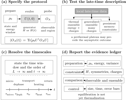
A nonequilibrium claim begins with the preparation, generator, and probe. The late-time description must then be tested against the relevant constraints, timescale window, finite-size behavior, and candidate ensemble. Equilibration is a dynamical statement; thermalization adds an ensemble-identification statement.

Exact Closed-System Dynamics

Consider first a finite system with a time-independent Hamiltonian. Write its spectral resolution as

$$H = \sum_E E P_E,$$

where $P_E$ projects onto the full eigenspace at energy $E$. Then

$$\rho(t) = \sum_{E,E'} e^{-i(E-E')t/\hbar} P_E\rho_0P_{E'}.$$

The expectation value is

$$\langle O\rangle_t = \sum_{E,E'} e^{-i(E-E')t/\hbar} \operatorname{Tr} \left( P_E\rho_0P_{E'}O \right).$$

Every time-dependent term is an interference term between distinct energies. Nonequilibrium dynamics is therefore governed by:

1. which energy amplitudes the preparation occupies;
2. the distribution and degeneracies of energy gaps;
3. the matrix elements of the chosen observable.

The density of states alone does not determine the dynamics.

Energy-basis form

For a nondegenerate spectrum with

$$H|n\rangle=E_n|n\rangle,$$

one obtains

$$\langle O\rangle_t = \sum_{m,n} \rho_{mn}(0) e^{-i(E_m-E_n)t/\hbar} O_{nm}.$$

The diagonal terms are constant. The off-diagonal terms oscillate with Bohr frequencies

$$\omega_{mn} = \frac{E_m-E_n}{\hbar}.$$

When many incommensurate frequencies contribute, their sum can become small for most times even though no term has been dissipated. This is dephasing.

The infinite-time average

Define the Cesàro time average

$$\overline{f} \equiv \lim_{T\to\infty} \frac{1}{T} \int_0^T f(t)\,dt,$$

when the limit exists. Since

$$\overline{ e^{-i(E-E')t/\hbar} } = \delta_{E,E'},$$

the time-averaged state is

$$\omega \equiv \overline{\rho(t)} = \sum_E P_E\rho_0P_E.$$

This is the dephased state or diagonal ensemble. The projector form is essential when $H$ has degeneracies: coherences within a degenerate energy eigenspace do not acquire a relative dynamical phase and therefore survive the time average.

For any bounded observable,

$$\overline{\langle O\rangle_t} = \operatorname{Tr}(\omega O).$$

This equality is exact under the stated finite-dimensional assumptions. It is not yet an equilibration theorem and not a thermalization theorem.

What the time average does not establish

Knowing the average does not show that $\langle O\rangle_t$ remains close to it. A signal can have the correct average while making large oscillations forever. The temporal variance

$$\sigma_O^2 \equiv \overline{ \left| \langle O\rangle_t - \operatorname{Tr}(\omega O) \right|^2 }$$

measures the residual fluctuations.

An effective number of occupied energy sectors is

$$d_{\mathrm{eff}} \equiv \frac{1}{\operatorname{Tr}(\omega^2)}.$$

A large $d_{\mathrm{eff}}$, together with sufficiently nondegenerate energy gaps and a restricted probe, can suppress time-averaged fluctuations. Those assumptions are substantive. Large Hilbert-space dimension by itself is not enough.

A Vocabulary of Late-Time Behavior

Several terms are often used interchangeably in informal prose but answer different questions.

Dephasing

Dephasing is cancellation among oscillatory contributions with different frequencies. It can occur under exact unitary evolution and requires no environment. It explains why a sum of coherent terms may become small for most times, but by itself it does not identify a thermal ensemble.

Relaxation

Relaxation is approach from an initial value toward a late-time value or regime. It is an observational description and should name:

• the observable or reduced state;
• the target value;
• the relaxation timescale;
• whether residual oscillations or algebraic tails remain.

Relaxation need not be monotonic.

Equilibration

An observable equilibrates if it is close to a reference value for most times after a transient. One operational criterion is

$$\begin{aligned} \mathcal B_\epsilon(T) &\equiv \left\{ t\in[0,T]: \right. \\ &\qquad \left. \left| \langle O\rangle_t - \operatorname{Tr}(\omega O) \right| > \epsilon \right\}, \\ \frac{ \mu\!\left(\mathcal B_\epsilon(T)\right) }{T} &\ll 1. \end{aligned}$$

for large $T$, where $\mu$ denotes the duration of the indicated set.

Equivalently, small temporal variance implies that large deviations occupy a small fraction of times. By Markov’s inequality,

$$\overline{ \mathbf 1_{ \{ |\langle O\rangle_t-\langle O\rangle_\omega| > \epsilon \} } } \leq \frac{\sigma_O^2}{\epsilon^2}.$$

This definition permits rare recurrences.

For a subsystem $A$, use the trace distance

$$D\!\left( \rho_A(t),\omega_A \right) = \frac{1}{2} \left\| \rho_A(t)-\omega_A \right\|_1.$$

Small trace distance means that every measurement confined to $A$ has nearly the same statistics in the two states.

Thermalization

Thermalization adds a second comparison:

$$\rho_A(t) \approx \omega_A \approx \rho_A^{\mathrm{th}}$$

for the specified subsystem or observable class and for most relevant late times.

The first approximation is equilibration. The second identifies the equilibrium state with a thermal ensemble constrained by energy and any additional global charges.

Thus:

$$\text{equilibration} \not\Rightarrow \text{thermalization}.$$

An integrable system may equilibrate to a generalized ensemble rather than an ordinary Gibbs state. A localized system may equilibrate imperfectly while retaining local memory. A finite two-level system may fail even to equilibrate.

Stationarity

A density operator is stationary under an autonomous Hamiltonian when

$$[H,\rho_{\mathrm{stat}}]=0.$$

The diagonal ensemble $\omega$ is stationary. The exact state $\rho(t)$ generally does not converge to $\omega$ in trace norm; its observables can nevertheless equilibrate around the values predicted by $\omega$.

Stationarity is therefore a property of a state or effective description, while equilibration is a property of observed time dependence.

Steady states

The phrase steady state has several meanings:

• an autonomous stationary state with time-independent observables;
• a dephased late-time regime in an isolated system;
• a periodic steady regime synchronized with a drive;
• an attracting fixed point of an open-system generator.

Only the last ordinarily involves genuine attraction in state space. In a finite isolated unitary system, distinct initial states cannot contract toward one density operator because unitary evolution preserves trace distance.

Prethermalization

A prethermal state is a long-lived intermediate regime controlled by approximate conservation laws or a separation of timescales. Schematically,

$$\tau_{\mathrm{local}} \ll t \ll \tau_*,$$

with observables close to an ensemble of an effective Hamiltonian or approximately conserved charges. At $t\sim\tau_*$, slower processes may drive the system toward another state.

The prefix “pre” matters: a plateau can be physically useful and parametrically long without being the asymptotic state.

Recurrence

Finite isolated quantum systems with discrete spectra exhibit arbitrarily close recurrences under broad conditions. The recurrence time often grows extremely rapidly with size, so recurrences can be irrelevant to laboratory times while remaining decisive for mathematical statements about $t\to\infty$ at fixed $L$.

Global Unitarity and Local Thermal Behavior

Suppose the full system begins in a pure state. Unitary evolution preserves purity:

$$\operatorname{Tr}\rho(t)^2 = \operatorname{Tr}\rho_0^2 = 1.$$

It also preserves the von Neumann entropy:

$$S(\rho(t)) = -\operatorname{Tr} \left[ \rho(t)\ln\rho(t) \right] = S(\rho_0).$$

There is no contradiction between these identities and local thermalization. For a bipartition $A\cup\bar A$,

$$\rho_A(t) = \operatorname{Tr}_{\bar A}\rho(t)$$

can become highly mixed because $A$ becomes entangled with $\bar A$. The lost local information remains encoded in nonlocal correlations of the full pure state.

Local indistinguishability

A precise local claim compares reduced states:

$$D \left( \rho_A(t), \rho_A^{\mathrm{th}} \right) \ll 1.$$

This implies

$$\begin{aligned} \Delta\rho_A(t) &\equiv \rho_A(t)-\rho_A^{\mathrm{th}}, \\ \Delta_{O_A}(t) &\equiv \left| \operatorname{Tr} \left[ O_A\Delta\rho_A(t) \right] \right|, \\ \Delta_{O_A}(t) &\leq 2\lVert O_A\rVert_\infty D \left( \rho_A(t), \rho_A^{\mathrm{th}} \right). \end{aligned}$$

Every bounded observable supported in $A$ then has nearly thermal statistics. A sufficiently nonlocal measurement on the full system can still reveal purity, conserved amplitudes, or detailed preparation information.

Entanglement entropy and thermal entropy

For a globally pure state,

$$S_A(t) = S_{\bar A}(t).$$

After a global quench, $S_A(t)$ often grows as entangled excitations cross the boundary of $A$. For a small region in a large thermalizing system, its late-time entanglement entropy can approach the thermodynamic entropy of the corresponding subsystem.

This agreement is conditional and local. The Thermal Entropy versus Entanglement Entropy page develops the exact distinctions, while Volume Laws explains when extensive entanglement scaling is expected.

Coarse graining is part of the statement

Irreversibility is not generated by silently replacing $\rho(t)$ with $\omega$. The physical statement is that a restricted observer, a local subsystem, a finite-resolution instrument, or a coarse-grained description cannot resolve the off-diagonal information for most relevant times.

The exact unitary state remains reversible. The effective description becomes autonomous only after the observable class and approximation are stated.

Which Ensemble Is the Candidate?

The late-time ensemble is constrained by quantities that the evolution preserves.

Energy alone

For an isolated autonomous system,

$$\frac{d}{dt} \langle H\rangle_t = 0.$$

If energy is the only relevant extensive conserved quantity within the chosen symmetry sector, a microcanonical state in a narrow shell around $\bar E$ is a natural candidate:

$$\rho_{\mathrm{mc}} = \frac{P_{[\bar E-\delta E,\bar E+\delta E]}} {\operatorname{Tr}P_{[\bar E-\delta E,\bar E+\delta E]}}.$$

For a small subsystem of a large short-range system away from problematic regimes, the microcanonical and canonical reduced states may agree:

$$\rho_A^{\mathrm{mc}} \approx \rho_A^\beta, \qquad \rho^\beta = \frac{e^{-\beta H}}{Z}.$$

The inverse temperature $\beta$ is fixed by matching the energy. This use of ensemble equivalence has assumptions involving subsystem size, interaction range, phase coexistence, and the thermodynamic limit; see Ensemble Equivalence.

Global charges and symmetry sectors

If $H$ commutes with particle number $N$, total magnetization, or another charge $Q_a$, the candidate state must reproduce those values. A generalized grand-canonical form is

$$\rho_{\mathrm{th}} = \frac{1}{Z} \exp \left[ -\beta \left( H-\sum_a\mu_a Q_a \right) \right].$$

It is usually cleaner to resolve exact symmetry sectors before testing spectral statistics or ETH. Mixing sectors can create spurious degeneracies and false indications of nonchaotic behavior.

Extensively many conserved quantities

An integrable model can possess an extensive family of independent or quasilocal charges $Q_j$. An ordinary Gibbs state retains too little information. A generalized Gibbs candidate has the form

$$\rho_{\mathrm{GGE}} = \frac{1}{Z_{\mathrm{GGE}}} \exp \left( -\sum_j\lambda_j Q_j \right),$$

with multipliers chosen to match the initial charge expectations.

This formula is only a template. Which charges are complete, local, or quasilocal is model dependent, and the order of limits can matter.

The diagonal ensemble as the exact memory ledger

The diagonal ensemble retains all initial populations in the energy basis:

$$\omega = \sum_E P_E\rho_0P_E.$$

A thermal or generalized ensemble is a compressed description of $\omega$ for a specified observable class. Thermalization succeeds when the omitted microscopic information is irrelevant to those observables in the controlled limit.

This hierarchy is useful:

$$\begin{gathered} \text{exact state }\rho(t) \\ \Downarrow\ \text{time averaging or equilibration} \\ \text{diagonal ensemble }\omega \\ \Downarrow\ \text{local ensemble equivalence} \\ \text{thermal or generalized ensemble}. \end{gathered}$$

The second arrow is the nontrivial thermalization step.

Why Generic Systems May Thermalize

The eigenstate thermalization hypothesis, or ETH, proposes that matrix elements of few-body observables in generic nonintegrable many-body energy eigenstates have a smooth thermodynamic structure. At overview depth, its two consequences are:

1. diagonal matrix elements $O_{nn}$ vary smoothly with energy, so a narrow energy distribution produces a thermal-looking mean;
2. off-diagonal matrix elements are sufficiently small and irregular that temporal fluctuations are suppressed in large systems.

This links the diagonal ensemble to a thermal ensemble for local probes. It is not a theorem for every local Hamiltonian, every eigenstate, or every initial condition.

One should distinguish:

• weak ETH: almost all eigenstates in an energy window are thermal for the chosen local probes;
• strong ETH: every eigenstate in the relevant window is thermal;
• dynamical thermalization: the chosen preparation has enough weight on appropriate eigenstates and sufficiently small late-time fluctuations.

Rare nonthermal eigenstates may invalidate strong ETH while leaving most preparations thermal. Conversely, a specially prepared state concentrated on rare eigenstates can fail to thermalize even when most eigenstates satisfy ETH.

Spectral level statistics, eigenvector structure, entanglement, and operator growth provide related diagnostics, but none alone is a definition of thermalization.

How Thermalization Can Fail

Failure is not one phenomenon. Different mechanisms preserve different kinds of information.

Integrability

Integrable systems have many conserved quantities that constrain late-time local observables. They may dephase and equilibrate while disagreeing with an ordinary Gibbs ensemble. A suitable generalized Gibbs ensemble can recover the local stationary data in models where the relevant charge set is known.

The one-dimensional quantum Newton’s-cradle experiment provided an influential example of strikingly weak relaxation in a nearly integrable Bose gas over thousands of collisions.

Localization and disorder

Disorder can inhibit transport and preserve local memory. Interactions can produce slow entanglement growth even when particle or energy transport is strongly suppressed. The stability and dimensional scope of many-body localization in thermodynamic systems remain active research questions; finite-size numerics and finite-time experiments must not be promoted automatically to an asymptotic phase statement.

Kinetic constraints and Hilbert-space fragmentation

Local constraints can split the accessible Hilbert space into dynamically disconnected or weakly connected sectors. A system can then fail to explore the full symmetry sector even without conventional integrability or quenched disorder.

The correct ensemble must be built on the actually accessible sector, not on the entire Hilbert space.

Quantum many-body scars

Some nonintegrable models contain atypical eigenstates embedded among otherwise thermal eigenstates. Initial states with large overlap on this sparse structure can show long-lived revivals and nonthermal dynamics.

Scars are a state-selective exception, not a blanket statement that the full spectrum is nonthermal. Persistent oscillations also require controls against finite-size effects, approximate symmetries, and ordinary weakly coupled modes.

Exact symmetries and degeneracies

If data from different symmetry sectors are mixed, conserved sector weights create apparent memory. Degenerate energies preserve within-eigenspace coherences in the diagonal ensemble. Both effects are exact and should be separated from more exotic mechanisms.

Small effective dimension

A preparation occupying only a few energy eigenstates has too few frequencies to dephase effectively. Even a Hamiltonian that thermalizes generic states need not thermalize such a preparation.

Hydrodynamic slow modes

Conserved densities can relax diffusively, superdiffusively, ballistically, or anomalously. Slow relaxation does not by itself imply failure of ETH. It may be the expected long-wavelength hydrodynamics of a thermalizing system.

Spreading Is Not One Velocity

After a local perturbation or global quench, several fronts can be defined.

Particle, spin, and energy transport

Conserved densities obey continuity equations such as

$$\partial_t n(\mathbf x,t) + \boldsymbol{\nabla}\cdot \mathbf j(\mathbf x,t) = 0.$$

Their long-wavelength dynamics can be ballistic, diffusive, subdiffusive, or superdiffusive depending on conservation laws, dimensionality, interactions, disorder, and integrability.

Transport asks how a conserved quantity moves. It is not identical to correlation or information spreading.

Correlation spreading

For local operators $A_X$ and $B_Y$ initially separated by distance $d(X,Y)$, a Lieb–Robinson bound for a short-range lattice Hamiltonian has the schematic form

$$\begin{aligned} \ell_{XY}(t) &\equiv d(X,Y)-v_{\mathrm{LR}}|t|, \\ \left\| [A_X(t),B_Y] \right\| &\leq C \exp \left[ -\mu\ell_{XY}(t) \right]. \end{aligned}$$

Outside the effective cone, influence is exponentially suppressed. The velocity $v_{\mathrm{LR}}$ is generally an upper bound, not the observed quasiparticle, correlation, transport, or butterfly velocity. The precise theorem and assumptions live at Lieb–Robinson Bound.

Entanglement spreading

Entanglement entropy across a cut can grow even when a conserved density barely moves. In one-dimensional generic systems after a global quench, a roughly linear growth regime is common before finite-size or subsystem-volume saturation:

$$S_A(t) \sim s_{\mathrm{ent}}v_E t.$$

This is a scaling template, not a universal law. Integrability, localization, conservation laws, long-range interactions, criticality, and inhomogeneity can change the form.

Operator spreading and scrambling

In the Heisenberg picture,

$$W(t) = e^{iHt/\hbar} W e^{-iHt/\hbar}$$

can acquire support on an expanding region. A squared commutator with a distant probe detects when the evolved operator becomes noncommuting there. Scrambling asks a stronger question about the delocalization of initially accessible quantum information.

Fast operator growth does not by itself prove local thermalization, and local thermalization does not require that every scrambling diagnostic has saturated.

A practical ordering

In a given model one may find different characteristic speeds:

$$\begin{gathered} v_{\mathrm{transport}}, \quad v_{\mathrm{corr}}, \quad v_E, \\ v_B, \quad v_{\mathrm{LR}}. \end{gathered}$$

There is no general rule that makes them equal. Report which front was measured and how it was extracted.

Driven Isolated Systems

For a closed system with explicit time dependence, energy need not be conserved. The instantaneous energy obeys

$$\frac{d}{dt} \langle H(t)\rangle = \left\langle \frac{\partial H(t)}{\partial t} \right\rangle.$$

To derive this, write

$$\begin{aligned} E(t) &\equiv \operatorname{Tr} \left[ \rho(t)H(t) \right], \\ \dot E(t) &= \operatorname{Tr} \left[ \dot\rho(t)H(t) \right] \\ &\quad + \operatorname{Tr} \left[ \rho(t)\dot H(t) \right]. \end{aligned}$$

The first term vanishes under

$$\dot\rho = -\frac{i}{\hbar} [H,\rho]$$

because the trace of a commutator is zero. The second term is the power injected by the drive.

Periodic driving

For

$$H(t+T)=H(t),$$

one-period evolution defines the Floquet operator

$$\begin{aligned} U_F &\equiv U(T,0), \\ &= \mathcal T \exp \left[ -\frac{i}{\hbar} \int_0^T H(t)\,dt \right]. \end{aligned}$$

Stroboscopic dynamics is

$$\rho(nT) = U_F^n\rho_0(U_F^\dagger)^n.$$

For generic interacting systems with a bounded local Hilbert space and no mechanism preventing absorption, periodic driving can lead toward an effectively infinite-temperature state at asymptotically late times. This statement has important exceptions and assumptions:

• exact or emergent conserved quantities can restrict heating;
• integrability can change the outcome;
• many-body localization has been proposed as a route to avoiding generic heating in suitable regimes, with stability questions requiring care;
• unbounded local spectra require a separate analysis;
• finite-frequency experiments may access only a long preasymptotic window.

High-frequency prethermalization

When the drive frequency $\Omega=2\pi/T$ is large compared with local energy scales, a truncated effective Hamiltonian $H_*$ can be approximately conserved:

$$U_F \approx \exp \left( -\frac{i}{\hbar} H_*T \right)$$

for times up to a heating scale $\tau_*$. In local bounded systems, rigorous results can make $\tau_*$ exponentially long in a suitable frequency-to-local-scale ratio:

$$\tau_* \gtrsim \tau_0 \exp \left( c\frac{\hbar\Omega}{J} \right),$$

with model- and theorem-dependent constants and norms.

The system can then relax with respect to $H_*$ before eventually absorbing substantial energy. This is Floquet prethermalization.

Driven steady regimes

An isolated periodically driven system has invertible unitary evolution. It therefore does not possess an attracting density operator in the same sense as a dissipative system. Nevertheless, local observables may:

• dephase to stroboscopically stationary values;
• synchronize into a $T$-periodic regime;
• remain in a long-lived prethermal plateau;
• heat slowly or rapidly.

The word “steady” should identify which of these is meant.

Open and Driven–Dissipative Systems

If the many-body system exchanges information or energy with an environment, its reduced state can obey a nonunitary equation. A Markovian example is

$$\begin{aligned} \dot\rho &= -\frac{i}{\hbar} [H,\rho] + \sum_\alpha \mathcal D[L_\alpha]\rho, \\ \mathcal D[L]\rho &\equiv L\rho L^\dagger - \frac{1}{2} \left\{ L^\dagger L,\rho \right\}. \end{aligned}$$

A steady state satisfies

$$\mathcal L(\rho_{\mathrm{ss}})=0.$$

Unlike closed unitary evolution, a dissipative semigroup can contract distinguishability and attract many initial states toward the same $\rho_{\mathrm{ss}}$.

Bath-induced thermalization, a nonequilibrium current-carrying steady state, and closed-system ETH thermalization are three different mechanisms. They can share a Gibbs-looking density operator in a limit without sharing the same dynamics or assumptions.

The system–bath approximations, complete positivity, detailed balance, and Liouvillian spectrum belong to Open Quantum Systems and the Markovian master-equation chapters.

The Timescale Ledger

Nonequilibrium behavior is rarely characterized by one relaxation time. A useful hierarchy is:

Scale	Typical role	What can set it
$\tau_{\mathrm{micro}}$	local oscillation or collision time	inverse hopping, exchange, interaction, or gap
$\tau_{\mathrm{deph}}$	cancellation of occupied Bohr frequencies	energy-width and gap distribution
$\tau_{\mathrm{local}}$	local equilibration	interactions, quasiparticle motion, operator growth
$\tau_{\mathrm{tr}}(L)$	transport across size $L$	ballistic, diffusive, or anomalous hydrodynamics
$\tau_{\mathrm{ent}}(L_A)$	entanglement across region $A$	entanglement velocity and subsystem geometry
$\tau_*$	prethermal lifetime	weak integrability breaking or high-frequency drive
$\tau_{\mathrm{heat}}$	substantial drive-induced heating	absorption rate and resonances
$\tau_{\mathrm{rec}}(L)$	finite-size recurrence	full many-body gap arithmetic

For a local energy scale $J$, dimensional analysis gives

$$\tau_{\mathrm{micro}} \sim \frac{\hbar}{J}.$$

This does not determine transport or thermalization times. A conserved density can require a size-dependent time

$$\tau_{\mathrm{tr}}(L) \sim \begin{cases} L/v, & \text{ballistic},\\ L^2/D, & \text{diffusive}, \end{cases}$$

where $v$ is a transport velocity and $D$ a diffusion constant.

Plateaus require two inequalities

To identify a prethermal or equilibrium plateau, show both:

$$t \gg \tau_{\mathrm{approach}}$$

and

$$t \ll \tau_{\mathrm{escape}}.$$

A flat-looking short trace is not enough. The lower inequality shows that the transient has ended; the upper inequality separates the plateau from recurrence, heating, finite-size saturation, or drift.

Order of limits

The expressions

$$\lim_{t\to\infty} \lim_{L\to\infty} \langle O\rangle_{L,t}$$

and

$$\lim_{L\to\infty} \lim_{t\to\infty} \langle O\rangle_{L,t}$$

need not agree. In the first expression, the thermodynamic limit is taken before the late-time limit. In the second, each finite system is evolved arbitrarily long first, exposing recurrences and exact finite-size structure.

Finite-size scaling at one fixed time is also insufficient. The useful object is often a joint window

$$\tau_{\mathrm{local}}(L) \ll t \ll \tau_{\mathrm{rec}}(L)$$

whose width grows with $L$.

Experimental and numerical windows

Experiments have decoherence, loss, calibration drift, and finite observation time. Numerics have finite size, bond dimension, timestep, truncation, and sampling error. A late-time claim should identify which boundary terminates the trustworthy window.

For tensor-network evolution, entanglement growth can make the reachable time shrink relative to the physical relaxation time. Failure to reach a plateau numerically is then an algorithmic limitation, not evidence of nonthermalization.

Worked Example: A Two-Level Quench That Does Not Equilibrate

Take

$$H = \frac{\hbar\Omega}{2} \sigma_x, \qquad \rho_0 = |\uparrow_z\rangle \langle\uparrow_z|.$$

The propagator is

$$U(t) = \cos\!\left(\frac{\Omega t}{2}\right)I - i\sin\!\left(\frac{\Omega t}{2}\right)\sigma_x.$$

The $z$-polarization is

$$\langle\sigma_z\rangle_t = \cos(\Omega t).$$

Its infinite-time average is zero:

$$\overline{\langle\sigma_z\rangle_t} = 0.$$

But its temporal variance is

$$\overline{ \left| \langle\sigma_z\rangle_t \right|^2 } = \frac{1}{2}.$$

The signal spends an order-one fraction of time far from its average. The diagonal ensemble predicts the mean but not equilibration.

The initial state has equal populations in the two energy eigenstates, so

$$d_{\mathrm{eff}}=2.$$

This example isolates the role of many frequencies: exact unitary evolution and a well-defined diagonal ensemble do not guarantee small fluctuations.

Worked Example: Dephasing Before Recurrence

Consider a normalized many-frequency signal

$$A_N(t) = \frac{1}{N} \sum_{k=1}^{N} \cos(\omega_k t).$$

For a dense set of frequencies distributed uniformly over

$$\omega \in [\omega_0-\Delta,\omega_0+\Delta],$$

the continuum limit gives

$$\begin{aligned} A_\infty(t) &= \frac{1}{2\Delta} \int_{\omega_0-\Delta}^{\omega_0+\Delta} \cos(\omega t)\,d\omega \\ &= \cos(\omega_0t) \frac{\sin(\Delta t)}{\Delta t}. \end{aligned}$$

The envelope decays as $1/t$:

$$\left| A_\infty(t) \right| \leq \frac{1}{|\Delta t|}$$

away from $t=0$. No microscopic oscillator has decayed; the sum has dephased.

At finite $N$, the signal is quasiperiodic and can recur. Increasing $N$ makes the continuum dephasing window longer and more convincing. This toy model displays why the thermodynamic and late-time limits may not commute.

Worked Example: Global Purity and Local Entropy

Begin with two qubits in $|00\rangle$ and evolve under

$$H = \hbar g \left( |00\rangle\langle11| + |11\rangle\langle00| \right).$$

The state is

$$|\psi(t)\rangle = \cos(gt)|00\rangle - i\sin(gt)|11\rangle.$$

It remains globally pure:

$$S \left( |\psi(t)\rangle\langle\psi(t)| \right) = 0.$$

The reduced state of the first qubit is

$$\rho_1(t) = \begin{pmatrix} \cos^2(gt) & 0\\ 0 & \sin^2(gt) \end{pmatrix}.$$

Its entropy is

$$S_1(t) = h_2 \left( \sin^2(gt) \right),$$

where

$$h_2(p) = -p\ln p - (1-p)\ln(1-p).$$

At $gt=\pi/4$, the reduced state is maximally mixed even though the full state is pure. In a many-body system, analogous entanglement with a large complement can make a small region locally thermal-looking for long times.

This two-qubit model demonstrates the mechanism but not thermodynamic irreversibility: it has exact revivals on the timescale $1/g$.

Worked Example: A Conserved Charge Rejects a Candidate Ensemble

Suppose

$$[H,Q]=0.$$

Then

$$\langle Q\rangle_t = \langle Q\rangle_0$$

for all $t$. Consider a candidate state $\rho_{\mathrm{cand}}$ with

$$\operatorname{Tr} \left( \rho_{\mathrm{cand}}Q \right) \neq \langle Q\rangle_0.$$

The candidate cannot describe thermalization for an observable class containing $Q$. More quantitatively,

$$\begin{aligned} \langle Q\rangle_{\mathrm{cand}} &\equiv \operatorname{Tr} \left( \rho_{\mathrm{cand}}Q \right), \\ \Delta_Q &\equiv \left| \langle Q\rangle_0 - \langle Q\rangle_{\mathrm{cand}} \right|, \\ \Delta_Q &\leq 2\lVert Q\rVert_\infty D \left( \rho(t), \rho_{\mathrm{cand}} \right). \end{aligned}$$

A nonzero charge mismatch therefore lower-bounds the trace distance:

$$D \left( \rho(t), \rho_{\mathrm{cand}} \right) \geq \frac{ \left| \langle Q\rangle_0 - \langle Q\rangle_{\mathrm{cand}} \right| }{ 2\lVert Q\rVert_\infty }.$$

In large systems one normally applies this logic to charge densities or finite regions, since the norm of an extensive $Q$ grows with system size.

Worked Example: Work Done by a Parameter Ramp

Let

$$H(t) = H_0+\lambda(t)V.$$

The power is

$$\frac{dE}{dt} = \dot\lambda(t) \langle V\rangle_t.$$

The net energy change is

$$\Delta E = \int_{t_i}^{t_f} \dot\lambda(t) \langle V\rangle_t\,dt.$$

The result depends on the evolving expectation value, not only on the endpoints of $\lambda$. Two ramps with the same endpoints can inject different energies because the state follows different trajectories.

For an instantaneous quench, the state is continuous across the quench while the Hamiltonian changes. The post-quench conserved energy is

$$E_f = \operatorname{Tr} \left( \rho_0 H_f \right),$$

not generally the ground-state energy of $H_f$ and not the expectation value of the pre-quench Hamiltonian.

Evidence Standards

“The system thermalizes” is incomplete. A reproducible claim should specify the following ledger.

State the claim operationally

A strong statement has the form:

For preparations in a declared family, observables in a declared class approach the predictions of a declared ensemble within tolerance $\epsilon$, for most times in a declared window, with controlled scaling in system size and numerical or experimental errors.

Changing any italicized ingredient can change the conclusion.

Audit the preparation

Report:

• energy density and energy variance under the evolution Hamiltonian;
• conserved charge densities and symmetry sector;
• spatial inhomogeneity and boundary conditions;
• purity or entropy when relevant;
• overlap with atypical states if that mechanism is invoked.

A narrow energy window supports comparison with a microcanonical ensemble. It does not prove that the occupied eigenstates are locally thermal.

Name the ensemble and match its constraints

For a Gibbs comparison, determine $\beta$ by matching energy and any chemical potentials by matching charges. For a GGE comparison, state the charge set. For an open steady state, state the generator and bath parameters.

Do not fit a separate effective temperature to every observable. A thermal ensemble makes joint predictions with one consistent set of intensive parameters.

Compare several observables

Use observables with different sensitivities:

• one-point densities;
• connected correlations at several separations;
• conserved currents or transport profiles;
• subsystem distributions;
• entanglement or purity when accessible.

Agreement of one coarse observable can be accidental or enforced by a conservation law.

Use an explicit distance or error measure

For an observable,

$$\delta_O(t) = \frac{ \left| \langle O\rangle_t - \langle O\rangle_{\mathrm{ens}} \right| }{ O_{\mathrm{scale}} }.$$

Choose $O_{\mathrm{scale}}$ independently of the fitted discrepancy and state it.

For reduced states, use trace distance, fidelity, or relative entropy. The quantum relative entropy

$$D_{\mathrm{rel}}(\rho\Vert\sigma) = \operatorname{Tr} \left[ \rho(\ln\rho-\ln\sigma) \right]$$

controls trace distance through the quantum Pinsker inequality:

$$D(\rho,\sigma) \leq \sqrt{ \frac{1}{2} D_{\mathrm{rel}}(\rho\Vert\sigma) }.$$

Full reduced-state tomography is expensive, so many experiments instead compare a controlled set of moments or correlators. That is a weaker, explicitly probe-dependent claim.

Resolve symmetries before spectral tests

Level statistics must be computed within irreducible symmetry sectors. Superposing independent sectors creates uncorrelated level sequences and can mimic Poisson statistics.

Likewise, ensemble comparisons must preserve exact sector weights unless a physical process changes them.

Demonstrate a time window

Show:

• approach to the plateau;
• fluctuations within the plateau;
• drift or lack of drift;
• the point at which decoherence, truncation, heating, or recurrence invalidates the interpretation.

Time averaging over a window should be accompanied by window-variation tests.

Scale system size and numerical control parameters

For exact diagonalization, vary $L$ and boundary conditions. For tensor networks, vary bond dimension and timestep. For stochastic methods, vary sample count. For experiments, vary coherence time, disorder realizations, calibration, and preparation fidelity where possible.

A plateau that moves substantially with $L$ is not yet a thermodynamic result.

Separate mechanism from phenomenology

Late-time Gibbs agreement is evidence of thermalization for the tested probes. It is not by itself proof of ETH. Persistent memory is evidence against that thermal description, but not by itself proof of integrability, localization, or scars.

Mechanism claims require their own diagnostics:

Proposed mechanism	Additional evidence
ETH	eigenstate matrix elements within resolved symmetry sectors
integrability	conserved-charge structure and GGE comparison
localization	transport suppression, local memory, entanglement dynamics, size and time scaling
scars	atypical eigenstates and state-selective overlap or revivals
prethermalization	parametrically separated drift and escape times, effective conserved quantity
Floquet heating	energy absorption and approach to the appropriate infinite-temperature values

Common Mistakes

• Equating a time average with equilibration. A mean can be well defined while fluctuations remain order one.
• Equating equilibration with thermalization. The equilibrium value may depend on more information than energy and global charges.
• Claiming convergence of the full finite closed-system state. Local observables can settle while $\rho(t)$ remains quasiperiodic.
• Calling dephasing decoherence. Dephasing among exact energy components can occur without an environment; environment-induced decoherence is a reduced-dynamics mechanism.
• Ignoring degeneracies. The diagonal ensemble is block diagonal in energy, not necessarily diagonal in an arbitrary basis inside a degenerate eigenspace.
• Fitting one temperature per observable. A genuine ensemble comparison uses one consistent parameter set.
• Mixing symmetry sectors in level statistics. This can manufacture apparent Poisson behavior.
• Using entropy growth without naming the entropy. Global von Neumann entropy is conserved under unitarity, while subsystem, diagonal, coarse-grained, and thermodynamic entropies answer different questions.
• Identifying a Lieb–Robinson speed with an observed front speed. The theorem generally supplies an upper envelope.
• Treating suppressed transport as proof of localization. Slow hydrodynamics, finite size, constraints, or long transients can imitate localization.
• Calling every plateau prethermal. A prethermal interpretation needs an escape timescale and an approximate conserved structure.
• Calling every persistent oscillation a scar. Weakly coupled modes, symmetry, integrability, and finite-size revivals must be excluded.
• Ignoring heating in a driven system. A useful prethermal Floquet regime can coexist with eventual energy absorption.
• Taking $t\to\infty$ at fixed finite size and interpreting the result as thermodynamic. State the order of limits.
• Inferring irreversibility from a truncated simulation. Entanglement truncation or finite bond dimension can suppress revivals and alter late-time values.

Chapter Roadmap

The subsequent pages divide the subject by canonical task:

Page	Canonical task
Quantum Quenches	sudden parameter changes, post-quench energy distributions, observable and entanglement dynamics
Relaxation and Thermalization	dephasing, subsystem equilibration, thermal ensembles, and conserved quantities
Eigenstate Thermalization Hypothesis	eigenstate matrix elements, diagonal smoothness, off-diagonal scaling, and exceptions
Integrability and Generalized Gibbs Ensembles Preview	extensive charges, Bethe-ansatz entry points, and GGE construction
Many-Body Localization Preview	disorder, interactions, local memory, entanglement growth, and frontier status
Prethermalization Preview	approximate conservation laws and parametrically long intermediate regimes
Quantum Chaos Preview	level statistics, random-matrix signatures, and the relation to ETH
Scrambling and OTOCs Preview	operator growth, squared commutators, information spreading, and QFT bridges
Loschmidt Echo and Dynamical Phase Transitions Preview	return amplitudes, Fisher zeros, rate functions, and interpretation caveats
Driven Many-Body Systems	work, energy absorption, heating, and driven–dissipative distinctions
Floquet Systems Preview	quasienergies, micromotion, effective Hamiltonians, and periodic phases

The overview supplies the common language. Each later page owns its detailed derivations, assumptions, and diagnostics.

Exercises

Exercise 1: Degenerate diagonal ensemble

Let

$$\begin{aligned} H &= E_0 \left( |1\rangle\langle1| + |2\rangle\langle2| \right) \\ &\quad + E_3|3\rangle\langle3|, \\ E_3 &\neq E_0. \end{aligned}$$

The initial state is

$$|\psi_0\rangle = \frac{1}{\sqrt3} \left( |1\rangle+|2\rangle+|3\rangle \right).$$

Find the time-averaged state. Which coherence survives?

Solution

The spectral projectors are

$$P_0 = |1\rangle\langle1| + |2\rangle\langle2|, \qquad P_3 = |3\rangle\langle3|.$$

The time-averaged state is

$$\omega = P_0\rho_0P_0 + P_3\rho_0P_3.$$

Expanding,

$$\begin{aligned} \omega &= \frac13 \left( |1\rangle\langle1| + |2\rangle\langle2| + |1\rangle\langle2| + |2\rangle\langle1| \right) \\ &\quad + \frac13 |3\rangle\langle3|. \end{aligned}$$

The coherence between $|1\rangle$ and $|2\rangle$ survives because those vectors have the same energy. Coherences connecting either of them to $|3\rangle$ oscillate with nonzero frequency and vanish in the time average.

Exercise 2: Time average is not equilibration

For the two-level quench with

$$\langle\sigma_z\rangle_t = \cos(\Omega t),$$

find the fraction of one period for which

$$\left| \langle\sigma_z\rangle_t \right| > \frac12.$$

Interpret the result.

Solution

Set $\theta=\Omega t$. Over one period $0\leq\theta<2\pi$, the condition is

$$|\cos\theta|>\frac12.$$

It holds on intervals of total length

$$\frac{4\pi}{3}.$$

The fraction is therefore

$$\frac{4\pi/3}{2\pi} = \frac23.$$

Although the infinite-time average is zero, the observable differs from that value by more than $1/2$ for two thirds of all times. The system does not equilibrate relative to this tolerance and observable.

Exercise 3: Width controls dephasing

For

$$A_\infty(t) = \cos(\omega_0t) \frac{\sin(\Delta t)}{\Delta t},$$

estimate the dephasing time and explain what happens as $\Delta\to0$.

Solution

The envelope first becomes small once

$$\Delta t \gtrsim 1.$$

Thus

$$\tau_{\mathrm{deph}} \sim \frac{1}{\Delta}.$$

As $\Delta\to0$, the frequency distribution collapses to one frequency. Using

$$\lim_{\Delta\to0} \frac{\sin(\Delta t)}{\Delta t} = 1,$$

one obtains

$$A_\infty(t) \to \cos(\omega_0t).$$

The dephasing time diverges and persistent oscillations return. A broad distribution of occupied frequencies, not merely long evolution, produces the decay.

Exercise 4: Local entropy from a pure state

For

$$|\psi(t)\rangle = \cos(gt)|00\rangle - i\sin(gt)|11\rangle,$$

find the times at which the first qubit is maximally mixed. What are the global and local entropies then?

Solution

The reduced state is maximally mixed when

$$\cos^2(gt) = \sin^2(gt) = \frac12.$$

Hence

$$gt = \frac{\pi}{4} + \frac{k\pi}{2}, \qquad k\in\mathbb Z.$$

At those times,

$$\rho_1 = \frac{I}{2}, \qquad S(\rho_1)=\ln2.$$

The full state remains pure, so

$$S \left( |\psi\rangle\langle\psi| \right) = 0.$$

The local entropy is entanglement entropy, not an increase of the global fine-grained entropy.

Exercise 5: Ensemble rejection by charge mismatch

Let $Q$ be a conserved operator with

$$\lVert Q\rVert_\infty=5.$$

The initial state has $\langle Q\rangle_0=2$, while a proposed ensemble has $\langle Q\rangle_{\mathrm{ens}}=-1$. Give a lower bound on the trace distance between the exact state and that ensemble.

Solution

The expectation mismatch is

$$\left| 2-(-1) \right| = 3.$$

Using

$$D(\rho,\sigma) \geq \frac{ |\langle Q\rangle_\rho-\langle Q\rangle_\sigma| }{ 2\lVert Q\rVert_\infty },$$

one finds

$$D \left( \rho(t),\rho_{\mathrm{ens}} \right) \geq \frac{3}{10}.$$

The proposed ensemble is operationally distinguishable by measuring $Q$ and cannot describe thermalization for an observable class that includes this charge.

Exercise 6: Energy injection under a cyclic protocol

For

$$H(t) = H_0+\lambda(t)V,$$

suppose $\lambda(t_i)=\lambda(t_f)=0$. Must $\Delta E$ vanish? Explain from the work formula.

Solution

No. The energy change is

$$\Delta E = \int_{t_i}^{t_f} \dot\lambda(t) \langle V\rangle_t\,dt.$$

Although the parameter returns to its initial value, $\langle V\rangle_t$ depends on the evolving state and generally has a phase lag relative to the drive. The integral can therefore be nonzero.

Only under additional conditions, such as a perfectly adiabatic cyclic protocol that returns the state to the same energy eigenspace up to phase, is zero net work guaranteed. Generic cyclic driving can heat the system.

Exercise 7: Distinguish three late-time claims

A finite isolated chain shows small fluctuations of a local density around the value predicted by its diagonal ensemble. That value disagrees with a Gibbs ensemble but agrees with a GGE. Classify the behavior.

Solution

The local density equilibrates because it remains close to its diagonal-ensemble value for most late times.

It does not thermalize to the ordinary Gibbs ensemble because that ensemble gives the wrong late-time value.

It is consistent with generalized thermalization or equilibration to a GGE, provided the proposed conserved charges are specified and the agreement extends beyond one fitted observable. The observation alone does not prove integrability; conserved-charge structure and broader tests are still required.

Exercise 8: Design a thermalization test

You simulate a nonintegrable spin chain after a product-state quench. List a minimal set of controls needed before claiming local thermalization.

Solution

A credible minimum is:

1. Resolve the exact symmetry sector and record the initial energy density and variance.
2. Construct a microcanonical or canonical comparison state with the same energy and charges.
3. Compare several local observables and connected correlations using one common temperature.
4. Show approach to a plateau and quantify temporal fluctuations over several windows.
5. Repeat for increasing system sizes and vary boundary conditions where practical.
6. Converge numerical controls such as timestep, Krylov tolerance, or tensor-network bond dimension.
7. Check that the observed time window lies before finite-size recurrence or truncation failure.
8. Separate the thermalization observation from any stronger ETH claim; the latter requires eigenstate-matrix-element evidence in resolved sectors.

No single item proves the result, but together they address preparation, ensemble, observable class, time window, size scaling, and numerical reliability.

References

• J. von Neumann, “Proof of the ergodic theorem and the $H$-theorem in quantum mechanics,” European Physical Journal H 35, 201–237, 2010 translation of the 1929 article, doi:10.1140/epjh/e2010-00008-5.
• J. M. Deutsch, “Quantum statistical mechanics in a closed system,” Physical Review A 43, 2046–2049, 1991, doi:10.1103/PhysRevA.43.2046.
• M. Srednicki, “Chaos and quantum thermalization,” Physical Review E 50, 888–901, 1994, doi:10.1103/PhysRevE.50.888.
• M. Rigol, V. Dunjko, V. Yurovsky, and M. Olshanii, “Relaxation in a completely integrable many-body quantum system: an ab initio study of the dynamics of the highly excited states of 1D lattice hard-core bosons,” Physical Review Letters 98, 050405, 2007, doi:10.1103/PhysRevLett.98.050405.
• M. Rigol, V. Dunjko, and M. Olshanii, “Thermalization and its mechanism for generic isolated quantum systems,” Nature 452, 854–858, 2008, doi:10.1038/nature06838.
• P. Reimann, “Foundation of statistical mechanics under experimentally realistic conditions,” Physical Review Letters 101, 190403, 2008, doi:10.1103/PhysRevLett.101.190403.
• N. Linden, S. Popescu, A. J. Short, and A. Winter, “Quantum mechanical evolution towards thermal equilibrium,” Physical Review E 79, 061103, 2009, doi:10.1103/PhysRevE.79.061103.
• A. J. Short and T. C. Farrelly, “Quantum equilibration in finite time,” New Journal of Physics 14, 013063, 2012, doi:10.1088/1367-2630/14/1/013063.
• A. Polkovnikov, K. Sengupta, A. Silva, and M. Vengalattore, “Colloquium: nonequilibrium dynamics of closed interacting quantum systems,” Reviews of Modern Physics 83, 863–883, 2011, doi:10.1103/RevModPhys.83.863.
• P. Calabrese and J. Cardy, “Time dependence of correlation functions following a quantum quench,” Physical Review Letters 96, 136801, 2006, doi:10.1103/PhysRevLett.96.136801.
• E. H. Lieb and D. W. Robinson, “The finite group velocity of quantum spin systems,” Communications in Mathematical Physics 28, 251–257, 1972, doi:10.1007/BF01645779.
• M. Cheneau et al., “Light-cone-like spreading of correlations in a quantum many-body system,” Nature 481, 484–487, 2012, doi:10.1038/nature10748.
• H. Kim and D. A. Huse, “Ballistic spreading of entanglement in a diffusive nonintegrable system,” Physical Review Letters 111, 127205, 2013, doi:10.1103/PhysRevLett.111.127205.
• T. Kinoshita, T. Wenger, and D. S. Weiss, “A quantum Newton’s cradle,” Nature 440, 900–903, 2006, doi:10.1038/nature04693.
• A. M. Kaufman et al., “Quantum thermalization through entanglement in an isolated many-body system,” Science 353, 794–800, 2016, doi:10.1126/science.aaf6725.
• D. M. Basko, I. L. Aleiner, and B. L. Altshuler, “Metal–insulator transition in a weakly interacting many-electron system with localized single-particle states,” Annals of Physics 321, 1126–1205, 2006, doi:10.1016/j.aop.2005.11.014.
• H. Bernien et al., “Probing many-body dynamics on a 51-atom quantum simulator,” Nature 551, 579–584, 2017, doi:10.1038/nature24622.
• C. J. Turner, A. A. Michailidis, D. A. Abanin, M. Serbyn, and Z. Papić, “Weak ergodicity breaking from quantum many-body scars,” Nature Physics 14, 745–749, 2018, doi:10.1038/s41567-018-0137-5.
• L. D’Alessio and M. Rigol, “Long-time behavior of isolated periodically driven interacting lattice systems,” Physical Review X 4, 041048, 2014, doi:10.1103/PhysRevX.4.041048.
• A. Lazarides, A. Das, and R. Moessner, “Equilibrium states of generic quantum systems subject to periodic driving,” Physical Review E 90, 012110, 2014, doi:10.1103/PhysRevE.90.012110.
• T. Mori, T. Kuwahara, and K. Saito, “Rigorous bound on energy absorption and generic relaxation in periodically driven quantum systems,” Physical Review Letters 116, 120401, 2016, doi:10.1103/PhysRevLett.116.120401.
• D. A. Abanin, W. De Roeck, W. W. Ho, and F. Huveneers, “Effective Hamiltonians, prethermalization, and slow energy absorption in periodically driven many-body systems,” Physical Review B 95, 014112, 2017, doi:10.1103/PhysRevB.95.014112.
• D. V. Else, B. Bauer, and C. Nayak, “Prethermal phases of matter protected by time-translation symmetry,” Physical Review X 7, 011026, 2017, doi:10.1103/PhysRevX.7.011026.
• L. D’Alessio, Y. Kafri, A. Polkovnikov, and M. Rigol, “From quantum chaos and eigenstate thermalization to statistical mechanics and thermodynamics,” Advances in Physics 65, 239–362, 2016, doi:10.1080/00018732.2016.1198134.

Further Connections

• Thermal Density Operators defines Gibbs states, temperature, and energy matching without assuming a dynamical route to equilibrium.
• Thermodynamic Limit develops size scaling, boundary effects, and noncommuting limits.
• Time-Dependent Correlations supplies the correlators used to track propagation, stationarity, and spectral relaxation.
• Real-Time Thermal Dynamics Preview explains why nonequilibrium initial data require more than equilibrium imaginary-time correlators.
• Schwinger–Keldysh Bridge carries that initial-value logic into doubled fields, influence actions, and nonequilibrium QFT.
• Many-Body Entanglement Overview organizes subsystem entropies and mixed-state measures.
• Operator Entanglement and Scrambling Preview separates operator support, operator entanglement, OTOCs, and recoverability.
• Boundaries distinguishes closed-system thermalization from interpretive foundations, open-system relaxation, and full nonequilibrium QFT.

Summary

The central inference chain is:

$$\begin{gathered} \text{specify }\rho_0,\ H(t),\ O_A,\ L, \\ \text{and the time and size limits}, \\ \Downarrow \\ \text{test equilibration relative to }\omega, \\ \Downarrow \\ \text{test }\omega_A\text{ against} \\ \text{a constrained ensemble}, \\ \Downarrow \\ \text{identify the mechanism} \\ \text{with independent diagnostics}. \end{gathered}$$

The durable distinctions are:

• unitary dephasing can produce local relaxation without destroying global information;
• equilibration means small late-time fluctuations, while thermalization identifies the equilibrium value with an ensemble;
• the diagonal ensemble is exact memory bookkeeping, whereas Gibbs and generalized ensembles are compressed local descriptions;
• integrability, localization, constraints, scars, symmetries, and small effective dimension preserve different kinds of memory;
• transport, correlation, entanglement, and operator fronts are not interchangeable;
• driven isolated systems can heat or prethermalize, while open systems can possess genuine attracting steady states;
• finite-size, finite-time, and order-of-limits controls are part of the result, not technical afterthoughts.