Driven Many-Body Systems

A driven many-body system is a quantum many-body system whose Hamiltonian, couplings, boundary conditions, or environmental channels are changed according to an externally specified protocol. Driving can prepare states, probe correlations, transport conserved quantities, engineer effective interactions, or stabilize nonequilibrium regimes. It can also inject energy until the desired structure is erased.

The central bookkeeping identity is simple. For a closed system with density operator $\rho(t)$ and explicitly time-dependent Hamiltonian $H(t)$,

$$\frac{d}{dt} \operatorname{Tr}\!\left[ \rho(t)H(t) \right] = \operatorname{Tr}\!\left[ \rho(t)\dot H(t) \right].$$

The right-hand side is the instantaneous power delivered by the prescribed drive. The difficult questions begin after this identity:

• Which energy is being monitored when the Hamiltonian itself changes?
• Is the drive local, boundary supported, or extensive?
• Does absorbed energy remain in the system, leave through a bath, or remove particles?
• Is the observed plateau a true asymptotic state, a prethermal window, or a finite-size recurrence?
• Does “infinite temperature” mean the whole Hilbert space or only a conserved symmetry sector?
• Is a measured decay really heating, or is it dephasing, loss, leakage, or imperfect detection?

This page develops the many-body answers. A useful drive is never characterized by frequency alone. Its amplitude, waveform, spatial support, duration, symmetries, initial state, bath coupling, and observation protocol all matter.

Purpose and Canonical Scope

This page owns the many-body interface among:

• time-dependent many-body Hamiltonians and extensive source terms;
• instantaneous and reference-energy ledgers;
• energy absorption per site and heating-rate diagnostics;
• local, boundary, and global driving;
• weak-drive spectral absorption and its breakdown;
• generic periodic heating and constrained infinite-temperature benchmarks;
• high-frequency prethermal windows as a heating-control mechanism;
• driven–dissipative energy balance and periodic steady regimes;
• numerical and experimental evidence standards.

Neighboring pages retain their canonical roles:

• Driven Closed Quantum Systems owns unitary propagation, elementary transition amplitudes, rotating-frame entry points, and control language for a general closed system.
• Time-Dependent Hamiltonians owns time ordering and the general propagator problem.
• Kubo Formula owns the full linear-response derivation, retarded correlators, contact terms, and transport limits.
• Work Distributions owns operational fluctuating-work distributions and their characteristic functions.
• Energy, Heat, and Work owns reduced-system thermodynamic conventions.
• Floquet Theorem in Quantum Mechanics owns the exact periodic spectral theorem, quasienergies, and micromotion.
• Floquet Systems Preview owns exponential quasienergy crowding, Floquet ETH, periodic engineering, and emergent many-body Floquet phases.
• High-Frequency Expansions owns Floquet–Magnus and van Vleck series, kick operators, resonant denominators, and optimal truncation.
• Prethermalization Preview owns the general two-timescale concept and evidence for an almost-conserved structure.
• Driven Open Systems owns time-dependent master equations, rotating frames, and drive-dressed dissipators.
• Steady States and Relaxation owns fixed points, Liouvillian gaps, dark subspaces, and metastability.

The present article uses those constructions to answer a different question: what becomes qualitatively new when a driven problem is extensive, interacting, and taken toward a thermodynamic limit?

The Minimal Many-Body Model

Write a driven Hamiltonian as

$$H(t) = H_0 + \sum_{a=1}^{M} \lambda_a(t)V_a.$$

Here $H_0$ is a reference Hamiltonian, $\lambda_a(t)$ are externally specified source amplitudes, and $V_a$ are the operators to which those sources couple. For a lattice system,

$$\begin{aligned} H_0 &= \sum_X h_X, \\ V_a &= \sum_X v_{a,X}, \end{aligned}$$

where $X$ labels sites, bonds, plaquettes, or other finite regions. Locality means that the terms have controlled range or decay and bounded local strength under a stated norm. It does not mean that the total operator norm stays finite as the volume $V$ grows.

Common sources include:

• a uniform magnetic field coupled to total magnetization;
• lattice-depth modulation coupled to kinetic and interaction energies;
• an electric field coupled through a vector potential or polarization;
• a moving trap or spatially varying potential;
• boundary pumping, particle injection, or loss;
• pulsed changes of interaction, tunneling, detuning, or geometry;
• coherent cavity or microwave drives;
• engineered dissipative channels.

The same waveform can represent very different thermodynamic perturbations depending on whether $V_a$ is local or extensive.

Closed evolution

For a retained closed system,

$$\dot\rho(t) = -\frac{i}{\hbar} [H(t),\rho(t)].$$

The evolution is unitary even though the system energy need not be conserved. The source that prescribes $\lambda_a(t)$ is outside the retained energy ledger. Calling the quantum system “closed” therefore does not mean that the combined laboratory, power supply, and quantum sample are closed.

Generalized forces

If the Hamiltonian is parameterized as $H(\boldsymbol\lambda)$, define the generalized force conjugate to $\lambda_a$ by

$$\mathcal F_a \equiv -\frac{\partial H}{\partial\lambda_a}.$$

The drive power is then

$$P_{\mathrm{drv}}(t) = -\sum_a \dot\lambda_a(t) \langle\mathcal F_a\rangle_t.$$

For the common convention

$$H(t)=H_0-f(t)B,$$

the generalized force is $B$ and

$$P_{\mathrm{drv}}(t) = -\dot f(t)\langle B\rangle_t.$$

Signs should be fixed from the Hamiltonian rather than remembered verbally.

Exact Energy Ledgers

Several inequivalent energies appear in driven work. A reliable analysis names the one being plotted.

Instantaneous system energy

Define

$$E_{\mathrm{inst}}(t) \equiv \operatorname{Tr}\!\left[ \rho(t)H(t) \right].$$

Differentiation gives

$$\begin{aligned} \dot E_{\mathrm{inst}} &= \operatorname{Tr}(\dot\rho H) + \operatorname{Tr}(\rho\dot H) \\ &= \operatorname{Tr}(\rho\dot H) \end{aligned}$$

for closed unitary evolution, because the trace of the commutator term vanishes. The average work performed on the retained system during $[t_0,t]$ is

$$W_{\mathrm{drv}}(t,t_0) = \int_{t_0}^{t} ds\, P_{\mathrm{drv}}(s).$$

This is an average energy transfer. It does not turn work into a state observable or define a unique work distribution.

Reference energy

Often the physically useful diagnostic is instead

$$E_0(t) \equiv \operatorname{Tr}\!\left[ \rho(t)H_0 \right].$$

For closed evolution,

$$\dot E_0(t) = -\frac{i}{\hbar} \operatorname{Tr}\!\left[ \rho(t)[H_0,H(t)] \right].$$

$E_0(t)$ measures excitation relative to a fixed reference, while $E_{\mathrm{inst}}(t)$ includes the changing source term. They coincide at the endpoints of a cyclic protocol only when the Hamiltonian returns to the same operator.

For periodic driving, useful choices include:

• the undriven energy $H_0$ sampled stroboscopically;
• the period-average Hamiltonian;
• an effective prethermal Hamiltonian $H_*$;
• experimentally reconstructed internal energy after ramping the drive off.

These choices answer different questions. A claim of “no heating” with respect to $H_*$ does not automatically imply constant $H_0$ energy, and vice versa.

Open-system energy balance

For a time-local reduced equation

$$\dot\rho = -\frac{i}{\hbar}[H(t),\rho] + \sum_\alpha \mathcal L_{\alpha,t}(\rho),$$

the same differentiation gives

$$\dot E_{\mathrm{inst}} = P_{\mathrm{drv}} + \sum_\alpha J_\alpha,$$

with

$$\begin{aligned} P_{\mathrm{drv}} &= \operatorname{Tr}(\rho\dot H), \\ J_\alpha &= \operatorname{Tr}\!\left[ H(t)\mathcal L_{\alpha,t}(\rho) \right]. \end{aligned}$$

Here $J_\alpha>0$ means energy enters the system from channel $\alpha$. This is the standard weak-coupling system-energy convention. At strong coupling, interaction energy and bath dressing can make the split model dependent.

A Drive Taxonomy

The word “drive” covers several physically distinct protocols.

Protocol	Defining feature	Natural question
sudden quench	parameter changes on an intrinsic short timescale	which final energies and excitations are populated?
finite ramp	parameter follows a path with a chosen speed	where does adiabatic following fail?
pulse	source has finite temporal support	what state or excitation packet remains afterward?
cyclic protocol	$H(t_f)=H(t_i)$	how much net work was absorbed or extracted?
periodic drive	$H(t+T)=H(t)$	does the system synchronize, prethermalize, or heat?
quasiperiodic drive	several incommensurate frequencies	how do multiple resonances and synthetic frequency dimensions enter?
stochastic drive	waveform has a noise spectrum	which transitions are activated by noise?
boundary drive	source or reservoir acts near an edge	what current and bulk profile result?
feedback drive	source depends on a measurement record	how do information and backaction alter the dynamics?

Quantum Quenches owns the sudden-protocol limit. Feedback and conditioned evolution belong to the measurement and control volume. This page focuses on externally prescribed many-body forcing and its energy consequences.

Local, Boundary, and Global Driving

Suppose

$$B_{\mathrm{glob}} = \sum_{x=1}^{V} b_x$$

is an extensive source operator. Under translation-invariant conditions,

$$\langle B_{\mathrm{glob}}\rangle = O(V),$$

so a fixed-amplitude source can deliver extensive power:

$$P_{\mathrm{drv}}=O(V).$$

The intensive object is $P_{\mathrm{drv}}/V$.

For a source supported on a fixed finite region,

$$B_{\mathrm{loc}} = \sum_{x\in R}b_x, \qquad |R|=O(1),$$

the injected energy at fixed time is ordinarily subextensive under bounded local dynamics. Locality then limits how rapidly the disturbed region can expand. A local drive may produce a persistent energy current or heat an ever-growing causal region, but it does not create a nonzero energy-density change throughout an infinite lattice at fixed time.

Boundary driving in $d$ spatial dimensions typically scales with area rather than volume:

$$P_{\partial} = O(L^{d-1}), \qquad V=O(L^d).$$

Whether a finite bulk gradient or current survives as $L\to\infty$ depends on transport, reservoirs, and the order of limits.

Symmetries and Dynamically Accessible Sectors

If an operator $Q$ satisfies

$$[H(t),Q]=0$$

for every time in the protocol, then its sector weights are conserved. A drive that preserves particle number cannot heat the system into a mixture of different particle-number sectors. A spin drive that preserves a parity can explore only the parity blocks occupied initially.

If $P_q$ projects onto a conserved sector with dimension

$$d_q=\operatorname{Tr}P_q,$$

the maximally mixed state in that sector is

$$\rho_{\infty,q} = \frac{P_q}{d_q}.$$

For an initial state with conserved sector weights

$$p_q=\operatorname{Tr}(P_q\rho_0),$$

the symmetry-constrained infinite-temperature benchmark is

$$\rho_{\infty}^{\mathrm{cons}} = \sum_q p_q \frac{P_q}{d_q}.$$

The drive may also possess selection rules without an exact conserved quantity. Selection rules suppress particular low-order transitions, but higher-order or interaction-assisted processes can remain.

What Heating Means

Heating is not simply “something decayed.” It is the redistribution of probability toward higher-energy states of a declared reference, or toward the appropriate high-entropy benchmark, due to energy absorption.

Intensive absorption measures

For a volume $V$, define the absorbed reference-energy density

$$q_0(t) \equiv \frac{ E_0(t)-E_0(t_0) }{V}.$$

Over a fitting window $[t_1,t_2]$, an average heating power density is

$$\overline p_0 = \frac{ E_0(t_2)-E_0(t_1) }{ V(t_2-t_1) }.$$

For a periodic drive, one often samples at $t_n=t_0+nT$ and writes

$$e_n \equiv \frac{1}{V} \operatorname{Tr}\!\left[ \rho(t_n)H_0 \right].$$

A normalized heating coordinate can be useful when the Hilbert space is bounded:

$$\mathcal Q_n = \frac{ e_n-e_0 }{ e_\infty-e_0 },$$

provided the denominator is nonzero and $e_\infty$ is computed in the correct conserved sector. Then $\mathcal Q_n=1$ means agreement with that energy benchmark, not proof that the full state is maximally mixed.

Heating, redistribution, loss, and dephasing

Four effects should be separated:

1. Absorption: the retained system gains reference energy.
2. Redistribution: interactions move energy among modes or quasiparticles.
3. Loss: particles or excitations leave the retained Hilbert space.
4. Dephasing: coherences decay while populations, and possibly energy, remain nearly fixed.

An atom-number decrease is not automatically heating. Contrast decay is not automatically energy absorption. A broadened spectrum can arise from interactions, noise, finite pulse duration, or loss. At least one calibrated energy-sensitive observable is needed.

Infinite temperature is sector dependent

For a finite lattice with bounded local Hilbert space and no conserved quantity beyond declared symmetry blocks, a generic interacting periodic drive may bring local observables toward the constrained trace state. The corresponding reference energy is

$$e_\infty = \frac{1}{V} \operatorname{Tr}\!\left[ \rho_{\infty}^{\mathrm{cons}}H_0 \right].$$

This statement concerns local observables or reduced states after dephasing. A globally pure closed state remains pure under unitary evolution:

$$\operatorname{Tr}\rho(t)^2 = \operatorname{Tr}\rho_0^2.$$

Global von Neumann entropy does not grow. Thermodynamic entropy growth enters through coarse graining, subsystems, diagonal ensembles, or coupling to an environment.

Unbounded local spectra

Bosonic lattices, continuum gases, and oscillators do not possess a normalizable identity state on the full Hilbert space. Their energy can grow without approaching a finite $e_\infty$, or particle loss and high-occupation processes can dominate first. A boson-number cutoff in a simulation manufactures a bounded spectrum; heating toward that cutoff is a convergence failure unless the cutoff is demonstrably irrelevant.

Weak-Drive Absorption

Take

$$H(t) = H_0-f(t)B$$

and suppose the initial state is stationary under $H_0$. The retarded susceptibility is

$$\chi^R_{BB}(t) = \frac{i}{\hbar} \theta(t) \left\langle [B(t),B(0)] \right\rangle_0.$$

With Fourier convention

$$\chi^R_{BB}(\omega) = \chi'_{BB}(\omega) + i\chi''_{BB}(\omega),$$

the absorptive part is $\chi''_{BB}$.

Harmonic source

For

$$f(t)=f_0\cos\omega t,$$

linear response gives

$$\begin{aligned} \delta\langle B(t)\rangle ={}& f_0 \left[ \chi'_{BB}(\omega)\cos\omega t \right. \\ &\left. \quad+ \chi''_{BB}(\omega)\sin\omega t \right]. \end{aligned}$$

Since $P_{\mathrm{drv}}=-\dot f\langle B\rangle$, the cycle-averaged absorbed power is

$$\overline P_{\mathrm{abs}} = \frac{f_0^2\omega}{2} \chi''_{BB}(\omega) + O(f_0^3).$$

For an extensive $B$, the susceptibility and power are extensive; divide by $V$ before taking a thermodynamic limit.

This formula is convention sensitive. Reversing the Fourier sign changes the sign assigned to $\chi''$, while the physical absorbed power remains unchanged.

Spectral representation

Let

$$H_0\lvert n\rangle = E_n\lvert n\rangle, \qquad \rho_0 = \sum_n p_n\lvert n\rangle\langle n\rvert.$$

Then

$$\begin{aligned} \chi''_{BB}(\omega) &= \frac{\pi}{\hbar} \sum_{m,n} w_{mn} \delta(\omega-\omega_{nm}), \\ w_{mn} &= (p_m-p_n)|B_{mn}|^2, \\ \omega_{nm} &= \frac{E_n-E_m}{\hbar}. \end{aligned}$$

For a positive-temperature Gibbs state and $\omega>0$, upward transitions carry greater initial weight than their reverse partners, so the net absorption is nonnegative. Interactions broaden and redistribute spectral weight in the thermodynamic limit, but they do not remove the need to specify the operator $B$.

Finite observation time

A drive applied for duration $\tau$ has frequency resolution of order

$$\delta\omega \sim \frac{1}{\tau}.$$

Finite-time spectra replace ideal delta peaks by window-dependent line shapes. The turn-on envelope can inject broadband energy, and abrupt switch-on can dominate the quantity attributed to steady harmonic absorption. Window functions, ramp duration, and sampling phase belong in the protocol specification.

Linear response is a controlled limit

The formula above requires a small source in the sense relevant to the measured time window. Breakdown can occur through:

• saturation of resonant transitions;
• multiphoton processes;
• drive-induced changes of the spectrum;
• nonperturbative avoided crossings;
• interaction-assisted redistribution;
• long times for which a small rate accumulates an order-one energy change;
• critical response that makes the thermodynamic and weak-source limits nonuniform.

A clean $f_0^2$ power law is evidence for the leading response regime. Its absence does not by itself identify which nonlinear mechanism has taken over.

Cyclic Work and Passivity

Suppose the protocol is cyclic,

$$H(t_f)=H(t_i)=H_0,$$

and the initial state is the Gibbs state

$$\rho_\beta = \frac{e^{-\beta H_0}}{Z}, \qquad \beta>0.$$

Closed evolution produces

$$\rho_f = U\rho_\beta U^\dagger.$$

The relative entropy satisfies

$$D(\rho_f\Vert\rho_\beta) \ge0.$$

Because unitary evolution preserves the von Neumann entropy,

$$\begin{aligned} D(\rho_f\Vert\rho_\beta) &= \beta \left[ \operatorname{Tr}(H_0\rho_f) - \operatorname{Tr}(H_0\rho_\beta) \right] \\ &= \beta W_{\mathrm{cyc}}. \end{aligned}$$

Therefore

$$W_{\mathrm{cyc}}\ge0.$$

A positive-temperature Gibbs state is passive: no cyclic unitary can lower its average energy. This does not mean that its energy rises monotonically during the cycle, nor does it forbid fluctuations in individual operational work records.

An active nonequilibrium state can yield $W_{\mathrm{cyc}}<0$, corresponding to work extraction. Ergotropy and Passive States owns the optimization problem and the distinction between passivity and complete passivity.

Beyond Linear Response

At finite amplitude, the drive dresses the states it is trying to excite. The response can contain harmonics, subharmonics, and multiphoton resonances:

$$E_n-E_m \simeq r\hbar\Omega, \qquad r\in\mathbb Z.$$

Interactions create many-body continua and allow an absorbed quantum to be redistributed among several excitations. Conversely, kinetic constraints or selection rules can force the lowest allowed process to high order.

Waveform harmonics

A periodic source can be expanded as

$$f(t) = \sum_{r\in\mathbb Z} f_r e^{-ir\Omega t}.$$

Even in linear response, each nonzero harmonic probes the susceptibility at $r\Omega$. A square pulse train and a sinusoid with the same fundamental frequency are therefore not equivalent. At nonlinear order, combinations of harmonics generate additional resonances.

Dense spectra

At fixed finite size, the many-body spectrum is discrete and the closed dynamics is quasiperiodic. As $V$ grows, the level spacing in a finite energy-density window is typically exponentially small. A drive frequency that avoids every exact transition in a small sample can intersect a dense set of many-body resonances in larger systems.

This is why the following limits need not commute:

$$\begin{aligned} &V\to\infty, &&t\to\infty, \\ &f_0\to0, &&\delta\omega\to0. \end{aligned}$$

A finite-size heating rate should be reported together with the spectral resolution and the time window over which it was inferred.

Periodic Driving as a Many-Body Regime

For

$$H(t+T)=H(t), \qquad \Omega=\frac{2\pi}{T},$$

the one-cycle unitary is

$$U_F(t_0) = \mathcal T \exp\!\left[ -\frac{i}{\hbar} \int_{t_0}^{t_0+T} H(s)\,ds \right].$$

Stroboscopic states obey

$$\rho_n = U_F^n \rho_0 (U_F^\dagger)^n.$$

The exact eigenphases, quasienergies, micromotion, and logarithm branches belong to the Floquet pages. Here the one-cycle map is used to organize energy absorption.

Why ordinary energy is not conserved

Quasienergy is defined modulo $\hbar\Omega$. It does not provide an extensive ordering analogous to the spectrum of a static local Hamiltonian. Repeated absorption and emission of drive quanta can connect states across the undriven many-body spectrum.

Under a common set of assumptions,

• interacting nonintegrable dynamics;
• bounded local Hilbert space;
• an extensive drive;
• no exact conservation law beyond declared sectors;
• no stable localization mechanism;
• sufficiently long times after the thermodynamic limit;

local observables can approach their constrained infinite-temperature values. This is a generic scenario, not a universal theorem for every periodic Hamiltonian.

High-frequency prethermal window

Let $J$ denote a local interaction scale, not the total many-body bandwidth. When

$$\frac{\hbar\Omega}{J} \gg1,$$

locality can suppress processes that absorb one drive quantum by requiring many coordinated local rearrangements. Under theorem-dependent boundedness and locality assumptions, there can exist a dressed effective Hamiltonian $H_*$ that changes only slowly, with a heating time scaling schematically as

$$\tau_* \gtrsim \frac{\hbar}{J} \exp\!\left( c\frac{\hbar\Omega}{J} \right).$$

The constant $c$, norm, prefactor, and allowed drive amplitude depend on the theorem and model. During

$$\tau_{\mathrm{rel}} \ll t \ll \tau_*,$$

the system may relax with respect to $H_*$ and exhibit a Floquet prethermal regime. Eventual heating can coexist with an exponentially useful observation window.

Comparing $\hbar\Omega$ with the total bandwidth, which grows with $V$, is the wrong thermodynamic criterion. The controlled comparison is with local energy scales and resonant matrix elements.

Low and intermediate frequencies

Low frequency does not guarantee adiabaticity in a many-body system. Small avoided crossings, gapless modes, critical points, and exponentially dense spectra can invalidate a naive adiabatic argument. Intermediate frequencies often contain the strongest resonances and the fastest heating.

A useful regime map asks separately about:

1. the drive frequency relative to local gaps and interaction scales;
2. the source amplitude relative to detunings;
3. the number of observed periods;
4. the system size;
5. the presence of baths or losses.

Mechanisms that alter heating

Heating can be suppressed, redirected, or delayed by:

• exact conserved quantities and symmetry sectors;
• integrability and stable quasiparticles;
• high-frequency prethermalization;
• destructive interference among drive paths;
• selection rules and kinetic constraints;
• disorder-enabled localization in regimes where it is stable;
• engineered dissipation that removes entropy or selected excitations;
• coupling only to a boundary or finite region;
• finite bandwidth or finite particle number;
• state-selective weak overlap with resonant sectors.

Each mechanism has its own diagnostic. A flat energy curve over ten periods is not a mechanism.

Isolated Long-Time Behavior

Closed unitary evolution does not produce an attracting global density operator. If

$$\rho(t) = U(t)\rho_0U^\dagger(t),$$

then trace distance between two initial states is preserved. Nevertheless, local observables can dephase and become synchronized with a periodic drive:

$$\langle O(t+T)\rangle \simeq \langle O(t)\rangle$$

after transients, within a chosen observation window.

Possible isolated regimes include:

• a stroboscopically stationary local state;
• a $T$-periodic local response including micromotion;
• a prethermal periodic regime governed by $H_*$;
• persistent quasiperiodic oscillations;
• subharmonic response under additional stability conditions;
• slow or rapid drift toward a constrained trace state;
• finite-size recurrences.

The word “steady” should say which object is steady: a stroboscopic observable, a reduced state, a diagonal ensemble, an effective temperature, or a dissipative fixed point.

Two-Step Spin-Chain Benchmark

A useful numerical benchmark alternates two noncommuting local Hamiltonians:

$$\begin{aligned} H_A &= J_z \sum_{j=1}^{V} \sigma_j^z\sigma_{j+1}^z, \\ H_B &= h_x \sum_{j=1}^{V} \sigma_j^x. \end{aligned}$$

Evolve with $H_A$ for time $T_A$ and then with $H_B$ for time $T_B$. The one-cycle operator is

$$U_F = e^{-iH_BT_B/\hbar} e^{-iH_AT_A/\hbar}.$$

The order matters because

$$[H_A,H_B]\ne0.$$

The global parity

$$\Pi_x = \prod_{j=1}^{V}\sigma_j^x$$

commutes with both steps. Heating benchmarks should therefore be computed in a fixed $\Pi_x$ sector or with the initial sector weights retained.

One may monitor the period-average reference Hamiltonian

$$\overline H = \frac{ T_AH_A+T_BH_B }{T_A+T_B}$$

through

$$e_n = \frac1V \operatorname{Tr}\!\left[ \rho_n\overline H \right].$$

This example cleanly tests:

• Trotter and time-order conventions;
• symmetry-resolved trace benchmarks;
• finite-size saturation;
• high-frequency plateaus;
• resonant parameter windows;
• entanglement-limited tensor-network times.

Special pulse angles can produce additional symmetries or integrability. Those points should not be used as evidence for generic heating without perturbing away from them.

Lattice-Modulation Spectroscopy

Consider the Fermi–Hubbard Hamiltonian

$$\begin{aligned} H_0 ={}& -J \sum_{\langle i,j\rangle,\sigma} \left( c_{i\sigma}^\dagger c_{j\sigma} + \text{h.c.} \right) \\ &+ U \sum_i n_{i\uparrow}n_{i\downarrow}. \end{aligned}$$

Modulating an optical lattice generally changes both $J$ and $U$:

$$\begin{aligned} J(t) &= J+\delta J\cos\omega t, \\ U(t) &= U+\delta U\cos\omega t. \end{aligned}$$

The perturbation couples to a specific combination of kinetic energy and double occupancy. In the weak-drive regime, the absorbed power probes the spectral function of that combination. Near strong coupling, features around $\hbar\omega\sim U$ can be associated with doublon–holon production, but the line shape also depends on bandwidth, temperature, filling, trap inhomogeneity, pulse duration, and interaction-assisted decay.

Doublon production is an informative proxy, not a universal thermometer. A complete analysis compares it with total energy, atom number, and at least one independent correlation observable.

Driven–Dissipative Many-Body Systems

A bath changes the asymptotic question. For a periodic Markovian generator,

$$\mathcal L_{t+T} = \mathcal L_t,$$

define the one-cycle quantum channel

$$\Phi_T = \mathcal T \exp\!\left[ \int_{t_0}^{t_0+T} \mathcal L_s\,ds \right].$$

A stroboscopic steady state satisfies

$$\Phi_T(\rho_*)=\rho_*.$$

The corresponding continuous-time periodic state is

$$\begin{aligned} \rho_{\mathrm{ps}}(t) &= \Phi(t,t_0)\rho_*, \\ \rho_{\mathrm{ps}}(t+T) &= \rho_{\mathrm{ps}}(t). \end{aligned}$$

It is a limit cycle in state space, not generally a time-independent density operator.

Cycle energy balance

In a periodic steady state,

$$E_{\mathrm{inst}}(t+T) = E_{\mathrm{inst}}(t).$$

Integrating the first law over one period gives

$$0 = W_{\mathrm{cyc}} + \sum_\alpha Q_{\alpha,\mathrm{cyc}},$$

where

$$\begin{aligned} W_{\mathrm{cyc}} &= \int_t^{t+T} ds\, P_{\mathrm{drv}}(s), \\ Q_{\alpha,\mathrm{cyc}} &= \int_t^{t+T} ds\, J_\alpha(s). \end{aligned}$$

Positive drive work can be balanced by negative heat into the system, meaning that energy flows out to the baths. A finite stationary energy therefore does not imply absence of absorption.

For thermodynamically consistent thermal generators, the cycle entropy production obeys

$$\Sigma_{\mathrm{cyc}} = -\sum_\alpha \frac{ Q_{\alpha,\mathrm{cyc}} }{ T_\alpha } \ge0,$$

because the system entropy returns to its initial value after one cycle. Entropy Production owns the assumptions behind this inequality.

The steady state is generally not Gibbs

Drive and dissipation can support currents, coherence in a rotating basis, bistability, metastability, spatial order, or persistent oscillations. The state is selected by the full generator, not by $H(t)$ alone:

$$\mathcal L_t \quad\text{or}\quad \Phi_T.$$

A bath does not automatically cool the system into the ground state of an effective Floquet Hamiltonian. The bath spectrum, coupling operators, drive dressing, secular approximation, and micromotion all affect transition rates.

Bare dissipators can be inconsistent

Appending a dissipator derived for $H_0$ to a strongly driven $H(t)$ can give incorrect stationary populations and energy currents. A controlled weak-coupling derivation may require transition operators in a rotating, dressed, or Floquet basis.

This issue becomes acute when:

• the Rabi frequency is comparable with relaxation rates;
• the drive changes Bohr frequencies substantially;
• quasienergy gaps are nearly degenerate;
• the bath has strong frequency dependence;
• the secular approximation separates the wrong transitions.

Driven Bose–Hubbard Cavity Lattice

A standard driven–dissipative model is a lattice of nonlinear lossy modes. In a rotating frame,

$$\begin{aligned} H_{\mathrm{rot}} ={}& -J \sum_{\langle i,j\rangle} \left( a_i^\dagger a_j+\text{h.c.} \right) \\ &+ \frac{U}{2} \sum_i n_i(n_i-1) -\hbar\Delta \sum_i n_i \\ &+ \sum_i \left( F_i a_i^\dagger+F_i^*a_i \right). \end{aligned}$$

Single-particle loss gives

$$\dot\rho = -\frac{i}{\hbar} [H_{\mathrm{rot}},\rho] + \kappa \sum_i \mathcal D[a_i]\rho.$$

The coherent source replenishes photons while loss removes them. The emitted flux is proportional to

$$\Phi_{\mathrm{out}} = \kappa \sum_i \langle n_i\rangle.$$

Interactions can produce sharp crossovers, metastability, and dissipative phase transitions as system size grows. The rotating-frame Hamiltonian is not a thermodynamic energy of the laboratory, and its lowest eigenstate is not generally the steady state. Input–output power and bath currents must be reconstructed in the physical frame or through a consistent rotating-frame thermodynamic convention.

Distinguishing Nonequilibrium Transitions

Several uses of “dynamical phase transition” coexist.

Phenomenon	Variable being varied	Singular object
equilibrium quantum phase transition	static coupling at $T=0$	ground-state energy or long-distance order
Loschmidt-rate DQPT	real evolution time	thermodynamic return-rate density
Floquet phase transition	drive parameter or eigenstate structure	quasienergy gap, stroboscopic order, or invariant
dissipative phase transition	drive, loss, or bath parameter	steady state and Liouvillian spectrum
long-time dynamical transition	control parameter	asymptotic order or trajectory regime

Loschmidt Echo and Dynamical Phase Transitions Preview owns return-rate singularities. A cusp in absorbed energy, a resonance, a bistable finite-size curve, and a closing Liouvillian gap are not interchangeable pieces of evidence.

A Regime and Evidence Ledger

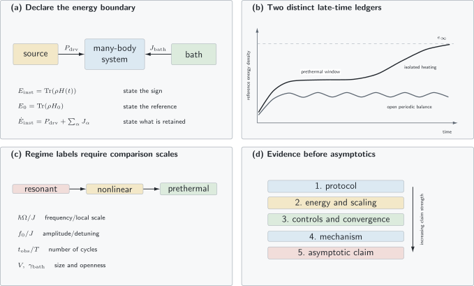
A driven-system claim begins with a declared source, reference energy, spatial scaling, and system boundary. An isolated bounded system may show a transient, a prethermal window, and eventual approach toward a symmetry-constrained trace benchmark; a driven open system can instead reach a periodic energy balance in which injected work leaves through baths. The lower panels separate regime labels from the evidence needed to support them.

The figure is a ledger, not a universal phase diagram. The ordering and even existence of the indicated windows depend on model, drive, initial state, dimension, and bath.

Numerical Methods

No single method controls all driven many-body regimes.

Method	Natural strength	Principal driven-system risk
exact diagonalization	full finite-size unitary or Floquet map	exponentially small sizes and misleading saturation
Krylov propagation	accurate finite-time pure-state dynamics	repeated long-time propagation and loss of orthogonality
product formulas	local time-dependent evolution	timestep resonances and incorrect pulse ordering
matrix-product states	one-dimensional local dynamics	entanglement growth and truncation-induced cooling
tensor networks for channels	one-dimensional open evolution	operator-space entanglement and positivity errors
quantum trajectories	sparse open-system propagation	sampling rare events and long correlation times
nonequilibrium Green functions	interacting spectra and driven materials	closure, memory, and self-energy consistency
dynamical mean-field theory	local correlations in high dimension	impurity solver and long-time convergence
kinetic equations	dilute or weak-scattering heating	uncontrolled closure near coherence or strong drive
semiclassical phase-space methods	large occupations or collective spins	missing nonclassical correlations

The method should be chosen from the claimed observable and timescale, not from the visual appeal of a long trajectory.

Numerical Convergence Ledger

A defensible simulation records:

1. Time resolution. Resolve the carrier, envelope, local interaction scale, and fastest bath rate.
2. Pulse order. Verify the convention for products such as $e^{-iH_BT_B}e^{-iH_AT_A}$.
3. Symmetry sector. Compare with the correct constrained trace value.
4. System size. Separate thermodynamic drift from finite-size saturation and recurrence.
5. Local cutoff. Increase boson or photon occupation cutoffs until heating observables converge.
6. Entanglement cutoff. Track discarded weight and repeat with larger bond dimension.
7. Integrator error. Check energy or norm conservation when the drive is off.
8. Drive phase. Distinguish stroboscopic observations from micromotion.
9. Fit window. Report how inferred heating rates change when early transients and late saturation are excluded.
10. Open-system checks. Verify trace, Hermiticity, positivity, trajectory convergence, and steady-state uniqueness assumptions.

An apparently suppressed heating rate can be produced by an insufficient local cutoff, bond-dimension truncation, an overly large timestep, or a finite-size plateau.

Experimental Diagnostics

Calibrate the source

The realized waveform may contain harmonics, phase noise, drift, and a turn-on transient absent from the intended protocol. Calibration should include:

• amplitude at the sample;
• carrier and harmonic content;
• envelope and phase;
• spatial inhomogeneity;
• timing jitter;
• parameter cross-couplings, such as simultaneous modulation of $J$ and $U$.

Measure more than one proxy

Useful observables include:

• internal or reference energy;
• double occupancy or defect density;
• momentum and density distributions;
• spin correlations and structure factors;
• entropy estimates or local thermometry;
• particle number and loss products;
• emitted photon flux and spectra;
• cycle-resolved power and bath currents.

Agreement of several observables with one equilibrium equation of state can support an effective-temperature interpretation. A single monotonic observable cannot.

Resolve the regime axes

A heating study should vary at least two of:

$$\Omega, \qquad f_0, \qquad V, \qquad t_{\mathrm{obs}}, \qquad \gamma_{\mathrm{bath}}.$$

Frequency scaling distinguishes resonant and high-frequency mechanisms. Amplitude scaling tests linear response and multiphoton order. Size scaling tests whether saturation is a finite-Hilbert-space effect. Bath scaling separates isolated absorption from steady energy throughput.

Separate loss from retained energy

If energetic particles leave a trap, the remaining cloud can cool even while the drive creates excitations. Conversely, loss can preferentially remove low-energy particles and heat the remainder. Report both total retained energy and particle number, or an energy per retained particle with the selection bias made explicit.

Evidence Ladder

A strong driven-many-body claim ascends the following ladder:

1. Declared protocol: write $H(t)$ or $\mathcal L_t$, the waveform, and the initial state.
2. Declared boundary: say whether the retained system is closed, lossy, or coupled to thermal reservoirs.
3. Declared energy: identify $H_{\mathrm{inst}}$, $H_0$, $\overline H$, or $H_*$.
4. Intensive normalization: state the volume, boundary area, particle number, or driven-region size.
5. Controls: turn off interactions, drive, bath, and known loss channels separately.
6. Scaling: vary frequency, amplitude, duration, and size.
7. Convergence: demonstrate numerical and experimental error budgets.
8. Mechanism: connect the trend to spectral weight, resonances, an almost-conserved quantity, or a bath balance.
9. Asymptotic restraint: distinguish observed windows from extrapolated infinite-time behavior.

The conclusion should match the rung reached. “Heating is suppressed over the observed window” can be authoritative when “the system never heats” is not.

Common Mistakes

• Treating explicit time dependence as proof of positive net absorption.
• Calling a drive “high frequency” without naming the local comparison scale.
• Comparing $\hbar\Omega$ with the extensive total bandwidth.
• Reporting raw energy rather than energy density for a global drive.
• Comparing a symmetry-preserving drive with the full-Hilbert-space trace state.
• Using instantaneous and reference energies interchangeably.
• Calling loss, dephasing, or contrast decay heating without an energy measurement.
• Inferring a thermal state from one effective thermometer.
• Assuming a finite isolated density operator converges to an attractor.
• Taking a finite-size saturation plateau as an infinite-temperature thermodynamic result.
• Claiming absence of heating before checking the bosonic occupation cutoff.
• Applying linear response after the absorbed energy is already order one.
• Ignoring the turn-on spectrum of a finite pulse.
• Treating quasienergy as an ordinary conserved extensive energy.
• Assuming integrability, localization, or a selection rule forbids all higher-order absorption.
• Calling a prethermal plateau a permanent phase without an escape-time analysis.
• Appending an undriven dissipator to a strong drive without rechecking its derivation.
• Calling a periodic open-system state time independent.
• Interpreting a rotating-frame Hamiltonian as the laboratory energy without qualification.
• Ignoring heat and particle currents when discussing a driven steady state.

Exercises

1. Exact closed-system power

Starting from

$$\dot\rho = -\frac{i}{\hbar}[H(t),\rho],$$

derive

$$\frac{d}{dt} \operatorname{Tr}[\rho H] = \operatorname{Tr}[\rho\dot H].$$

Why does this not contradict unitarity?

Solution

Differentiate the expectation value:

$$\frac{d}{dt} \operatorname{Tr}(\rho H) = \operatorname{Tr}(\dot\rho H) + \operatorname{Tr}(\rho\dot H).$$

The first term is

$$\begin{aligned} \operatorname{Tr}(\dot\rho H) &= -\frac{i}{\hbar} \operatorname{Tr}([H,\rho]H) \\ &= -\frac{i}{\hbar} \operatorname{Tr}(\rho[H,H]) \\ &=0. \end{aligned}$$

Only the explicit parameter dependence remains. Unitarity preserves inner products, spectrum of $\rho$, and global von Neumann entropy. It does not conserve the expectation of an explicitly time-dependent Hamiltonian.

2. Harmonic absorption

Let

$$H(t)=H_0-f_0\cos(\omega t)B$$

and suppose

$$\delta\langle B(t)\rangle = f_0 \left[ \chi'\cos\omega t + \chi''\sin\omega t \right].$$

Compute the cycle-averaged power to quadratic order in $f_0$.

Solution

The power is

$$P(t) = -\dot f(t)\langle B(t)\rangle.$$

Since

$$-\dot f(t) = f_0\omega\sin\omega t,$$

the source-independent expectation averages to zero when multiplied by a sinusoid. The in-phase response also averages to zero:

$$\overline{ \sin\omega t\cos\omega t } =0.$$

The out-of-phase part gives

$$\overline{ \sin^2\omega t } = \frac12,$$

so

$$\overline P = \frac{f_0^2\omega}{2} \chi''.$$

The sign of the symbol $\chi''$ depends on the Fourier convention; the physical absorbed power does not.

3. Cyclic passivity

Let $\rho_\beta=e^{-\beta H_0}/Z$ with $\beta>0$, and let a cyclic unitary produce $\rho_f=U\rho_\beta U^\dagger$. Use relative entropy to show that the average cyclic work is nonnegative.

Solution

Start from

$$D(\rho_f\Vert\rho_\beta) = \operatorname{Tr} \left[ \rho_f(\ln\rho_f-\ln\rho_\beta) \right] \ge0.$$

Because $\rho_f$ is unitarily related to $\rho_\beta$,

$$\operatorname{Tr}(\rho_f\ln\rho_f) = \operatorname{Tr}(\rho_\beta\ln\rho_\beta).$$

Using

$$\ln\rho_\beta = -\beta H_0-\ln Z,$$

the normalization terms cancel and

$$D(\rho_f\Vert\rho_\beta) = \beta \operatorname{Tr} \left[ H_0(\rho_f-\rho_\beta) \right].$$

The bracket is the average work for a cyclic protocol. Therefore

$$W_{\mathrm{cyc}} = \frac{1}{\beta} D(\rho_f\Vert\rho_\beta) \ge0.$$

4. Symmetry-constrained infinite temperature

A periodic spin chain conserves parity $\Pi$ with projectors $P_\pm$. The initial state has sector weights $p_\pm$. Write the constrained trace state and the corresponding infinite-temperature value of an observable $O$.

Solution

Let

$$d_\pm = \operatorname{Tr}P_\pm.$$

The sector weights cannot change, so the appropriate trace state is

$$\rho_\infty^{\mathrm{cons}} = p_+ \frac{P_+}{d_+} + p_- \frac{P_-}{d_-}.$$

Therefore

$$\langle O\rangle_\infty = p_+ \frac{ \operatorname{Tr}(P_+O) }{d_+} + p_- \frac{ \operatorname{Tr}(P_-O) }{d_-}.$$

Using $\operatorname{Tr}(O)/\dim\mathcal H$ is correct only when the sector weights match the full trace state or when the observable has the same normalized trace in both sectors.

5. Local versus global power

Let $B_{\mathrm{glob}}=\sum_{x=1}^{V}b_x$ and suppose connected correlations remain summable. Compare the expected scaling of absorbed power for $H_{\mathrm{drv}}=-f(t)B_{\mathrm{glob}}$ with a drive supported on $O(1)$ sites.

Solution

For a homogeneous global drive, both $\langle B_{\mathrm{glob}}\rangle$ and the extensive susceptibility scale as $V$. Thus

$$P_{\mathrm{glob}} = O(V), \qquad \frac{P_{\mathrm{glob}}}{V} = O(1).$$

For a source supported on a fixed region with bounded local operators, the instantaneous power is $O(1)$. At fixed time, the total injected energy is therefore subextensive and its contribution to the energy density vanishes as $V\to\infty$.

At long times a local source can heat a growing region or sustain a current into the bulk. The fixed-time statement does not determine the limit obtained by taking $t\to\infty$ first.

6. A commuting cyclic drive

Consider

$$H(t)=a(t)H_0, \qquad a(t_f)=a(t_i).$$

Show that the populations in the $H_0$ eigenbasis do not change and that a cyclic protocol produces no net reference-energy absorption.

Solution

Hamiltonians at all times commute:

$$[H(t),H(t')]=0.$$

The propagator is

$$U(t_f,t_i) = \exp\!\left[ -\frac{iH_0}{\hbar} \int_{t_i}^{t_f} a(s)\,ds \right].$$

$U$ is a function of $H_0$, so it commutes with every projector onto an $H_0$ eigenspace. Populations are unchanged, and

$$\operatorname{Tr}(\rho_fH_0) = \operatorname{Tr}(\rho_iH_0).$$

The instantaneous energy can vary because $a(t)$ varies, but it returns to its initial value when the Hamiltonian and reference coincide again. Explicit time dependence alone is not sufficient for heating.

7. Periodic open-system balance

A periodic Markovian system reaches $\rho_{\mathrm{ps}}(t+T)=\rho_{\mathrm{ps}}(t)$. Show that the drive work and bath heats sum to zero over one cycle.

Solution

The exact reduced-system balance is

$$\dot E = P_{\mathrm{drv}} + \sum_\alpha J_\alpha.$$

Integrate over one period:

$$\begin{aligned} \Delta E_T &\equiv E(t+T)-E(t), \\ \Delta E_T &= W_{\mathrm{cyc}} + \sum_\alpha Q_{\alpha,\mathrm{cyc}}, \\ W_{\mathrm{cyc}} &\equiv \int_t^{t+T}ds\, P_{\mathrm{drv}}(s), \\ Q_{\alpha,\mathrm{cyc}} &\equiv \int_t^{t+T}ds\, J_\alpha(s). \end{aligned}$$

Periodicity makes $\Delta E_T=0$, so

$$W_{\mathrm{cyc}} + \sum_\alpha Q_{\alpha,\mathrm{cyc}} =0.$$

A constant cycle-averaged energy can therefore coexist with continuous positive work input and equal energy flow out to the baths.

8. Design a heating audit

An experiment reports that a driven interacting lattice “does not heat” for $50$ periods because a density-wave contrast remains constant. Give a minimal audit needed to support or revise the claim.

Solution

A minimal audit would:

• write the realized drive waveform, including harmonics and turn-on;
• identify whether the drive is global, local, or boundary supported;
• measure a calibrated reference energy or several energy-sensitive observables;
• track particle number and loss products separately;
• vary drive frequency and amplitude;
• extend the observation time and vary system size where possible;
• compare with the correct symmetry-constrained trace benchmark;
• test an interaction-off or drive-off control;
• verify that contrast is not protected by a conservation law or selection rule;
• compare with converged numerics, including local cutoff and timestep checks;
• fit heating rates over several windows after excluding transients and saturation.

The data may support “no resolved heating over $50$ periods within sensitivity” or “a prethermal plateau consistent with suppressed heating.” A constant contrast alone does not establish either zero absorption or infinite lifetime.

Research Status

Several conclusions are well established under stated assumptions:

• a time-dependent Hamiltonian supplies exact drive power through $\langle\dot H\rangle$;
• weak harmonic absorption is controlled by the dissipative susceptibility;
• positive-temperature Gibbs states are passive under cyclic unitary driving;
• generic interacting periodic systems with bounded local Hilbert spaces can heat toward symmetry-constrained trace values;
• local high-frequency drives can exhibit exponentially long prethermal windows;
• finite systems can show saturation and recurrences unrelated to a thermodynamic heating law;
• baths can balance injected work and stabilize nonequilibrium steady states or limit cycles;
• drive-dressed system–bath coupling matters for thermodynamic consistency.

Active research includes:

• quantitative heating rates beyond linear response;
• stability of nonheating regimes in higher dimensions and unbounded systems;
• rare many-body resonances at very high frequency;
• driven phases that survive realistic noise and baths;
• controlled thermodynamics of strongly coupled or non-Markovian driven systems;
• scalable certification of dissipative many-body steady states;
• extracting many-body absorption from short, noisy quantum-simulator data;
• first-principles treatment of correlated driven materials.

Claims in the second list should carry the model, dimension, interaction range, drive, bath, and observation window with them.

Further Connections

• Nonequilibrium Overview — the shared initial-value and energy-balance language.
• Quantum Quenches — sudden driving and final-energy distributions.
• Relaxation and Thermalization — dephasing and local ensemble agreement after the drive.
• Prethermalization Preview — almost-conserved quantities and separated clocks.
• Many-Body Localization Preview — disorder-enabled memory and stability cautions.
• Kubo Formula — canonical many-body linear response.
• Fluctuation–Dissipation Theorem — equilibrium noise and absorption.
• High-Frequency Expansions — effective Hamiltonians, micromotion, and optimal truncation.
• Floquet–Magnus Expansion — the direct one-period Magnus construction.
• Floquet Operators — eigenphases, branches, and stroboscopic maps.
• Work Distributions — operational fluctuations of work.
• Driven Open Systems — time-dependent generators and control validity.
• Steady States and Relaxation — Liouvillian fixed points, gaps, and metastability.
• Driven-Dissipative Matter — material platforms, polariton fluids, output observables, and transition evidence.
• Vortex Matter, Pinning, and Flux Flow — applies drive, power-balance, heating, bath, and observation-window discipline to superconducting vortex motion while retaining the material force, pinning, creep, and flux-flow ledger.
• Entropy Production — heat-current conventions and irreversible balance.

References

• R. Kubo, “Statistical-mechanical theory of irreversible processes. I. General theory and simple applications to magnetic and conduction problems,” Journal of the Physical Society of Japan 12, 570–586 (1957).
• W. Pusz and S. L. Woronowicz, “Passive states and KMS states for general quantum systems,” Communications in Mathematical Physics 58, 273–290 (1978).
• A. Lenard, “Thermodynamical proof of the Gibbs formula for elementary quantum systems,” Journal of Statistical Physics 19, 575–586 (1978).
• H. Spohn, “Entropy production for quantum dynamical semigroups,” Journal of Mathematical Physics 19, 1227–1230 (1978).
• S. Diehl, A. Micheli, A. Kantian, B. Kraus, H. P. Büchler, and P. Zoller, “Quantum states and phases in driven open quantum systems with cold atoms,” Nature Physics 4, 878–883 (2008).
• T. Oka and H. Aoki, “Photovoltaic Hall effect in graphene,” Physical Review B 79, 081406(R) (2009).
• A. Lazarides, A. Das, and R. Moessner, “Equilibrium states of generic quantum systems subject to periodic driving,” Physical Review E 90, 012110 (2014).
• L. D’Alessio and M. Rigol, “Long-time behavior of isolated periodically driven interacting lattice systems,” Physical Review X 4, 041048 (2014).
• P. Ponte, A. Chandran, Z. Papić, and D. A. Abanin, “Periodically driven ergodic and many-body localized quantum systems,” Annals of Physics 353, 196–204 (2015).
• P. Ponte, Z. Papić, F. Huveneers, and D. A. Abanin, “Many-body localization in periodically driven systems,” Physical Review Letters 114, 140401 (2015).
• D. A. Abanin, W. De Roeck, and F. Huveneers, “Exponentially slow heating in periodically driven many-body systems,” Physical Review Letters 115, 256803 (2015).
• T. Kuwahara, T. Mori, and K. Saito, “Floquet–Magnus theory and generic transient dynamics in periodically driven many-body quantum systems,” Annals of Physics 367, 96–124 (2016).
• T. Mori, T. Kuwahara, and K. Saito, “Rigorous bound on energy absorption and generic relaxation in periodically driven quantum systems,” Physical Review Letters 116, 120401 (2016).
• D. A. Abanin, W. De Roeck, W. W. Ho, and F. Huveneers, “Effective Hamiltonians, prethermalization, and slow energy absorption in periodically driven many-body systems,” Physical Review B 95, 014112 (2017).
• M. Reitter, J. Näger, K. Wintersperger, C. Sträter, I. Bloch, A. Eckardt, and U. Schneider, “Interaction dependent heating and atom loss in a periodically driven optical lattice,” Physical Review Letters 119, 200402 (2017).
• P. Bordia, H. Lüschen, U. Schneider, M. Knap, and I. Bloch, “Periodically driving a many-body localized quantum system,” Nature Physics 13, 460–464 (2017).
• M. Fitzpatrick, N. M. Sundaresan, A. C. Y. Li, J. Koch, and A. A. Houck, “Observation of a dissipative phase transition in a one-dimensional circuit QED lattice,” Physical Review X 7, 011016 (2017).
• M. Foss-Feig, J. T. Young, V. V. Albert, A. V. Gorshkov, and M. F. Maghrebi, “Solvable family of driven-dissipative many-body systems,” Physical Review Letters 119, 190402 (2017).
• K. Mallayya and M. Rigol, “Heating rates in periodically driven strongly interacting quantum many-body systems,” Physical Review Letters 123, 240603 (2019).
• K. Sandholzer, Y. Murakami, F. Görg, J. Minguzzi, M. Messer, R. Desbuquois, M. Eckstein, P. Werner, and T. Esslinger, “Quantum simulation meets nonequilibrium dynamical mean-field theory: exploring the periodically driven, strongly correlated Fermi–Hubbard model,” Physical Review Letters 123, 193602 (2019).
• A. Rubio-Abadal, M. Ippoliti, S. Hollerith, D. Wei, J. Rui, S. L. Sondhi, V. Khemani, C. Gross, and I. Bloch, “Floquet prethermalization in a Bose–Hubbard system,” Physical Review X 10, 021044 (2020).
• K. Viebahn, J. Minguzzi, K. Sandholzer, A.-S. Walter, M. Sajnani, F. Görg, and T. Esslinger, “Suppressing dissipation in a Floquet–Hubbard system,” Physical Review X 11, 011057 (2021).
• T. Mori, “Heating rates under fast periodic driving beyond linear response,” Physical Review Letters 128, 050604 (2022).
• A. Rakcheev and A. M. Läuchli, “Estimating heating times in periodically driven quantum many-body systems via avoided crossing spectroscopy,” Physical Review Research 4, 043174 (2022).

Summary

• The exact drive power of a closed system is $\langle\dot H\rangle$, but the physically useful heating diagnostic may instead be energy relative to $H_0$, a period average, or a prethermal $H_*$.
• Local, boundary, and global drives have different thermodynamic scaling.
• Weak harmonic absorption is governed by the absorptive susceptibility; finite amplitude introduces dressing, saturation, and multiphoton processes.
• Gibbs states are passive under cyclic unitary protocols, so their average cyclic work is nonnegative.
• Generic periodic many-body heating toward a constrained trace state requires bounded local Hilbert space and the absence of mechanisms that prevent absorption.
• High-frequency driving can produce exponentially long prethermal windows without guaranteeing eternal stability.
• A driven open system can maintain finite energy while continuously converting drive work into heat flowing to baths.
• Heating claims require calibrated sources, declared energy conventions, symmetry-aware benchmarks, scaling, convergence, and separation from loss and dephasing.