Kubo Formula

The Kubo formula gives the first change in a many-body observable produced by a weak external source. Driven Many-Body Systems owns the corresponding absorption power, nonlinear breakdown, heating, and bath-balance interpretation. If the perturbation is

$$H_{\mathrm{pert}}(t) = -f(t)B,$$

then the response of an observable $A$ is

$$\delta\langle A(t)\rangle = \int_{-\infty}^{\infty} dt'\, \chi^R_{AB}(t,t') f(t') + O(f^2),$$

with retarded susceptibility

$$\chi^R_{AB}(t,t') = \frac{i}{\hbar} \theta(t-t') \left\langle [A_H(t),B_H(t')] \right\rangle_0.$$

The sign is tied to the explicit choice $H_{\mathrm{pert}}=-fB$. The step function enforces causality. The commutator measures the difference between the two operator orders. The expectation value is taken in the unperturbed reference state, and the Heisenberg operators evolve with the unperturbed Hamiltonian.

This identity is exact to first order in the source. The hard work in a many-body application is specifying the correct source, detector, ensemble, current or density operators, contact terms, Fourier convention, boundary conditions, and order of limits.

Canonical Scope

This page is the canonical home for the generic many-body Kubo formula. It owns:

• source-coupled perturbations and the retarded-commutator derivation;
• space- and time-dependent response kernels;
• equilibrium Lehmann representations;
• reactive and dissipative response;
• static versus dynamical susceptibilities;
• explicit source dependence and contact terms;
• magnetic, density, and electrical-conductivity examples;
• finite-size, zero-frequency, and thermodynamic-limit cautions.

Time-Dependent Correlations owns ordinary unequal-time products, their positive Lehmann measures, thermal detailed balance, dephasing, and recurrence. Green Functions and Response Preview owns the introductory Green-function bridge and harmonic-oscillator example. Linear Response Preview owns the transition-amplitude, golden-rule, and finite-time dictionary. This page starts from those ingredients and develops the many-body response calculation.

Green Functions in Many-Body QM owns normal single-particle propagators. Its retarded fermionic function uses an anticommutator and connects $N$ to $N\pm1$ sectors; it is not the observable susceptibility derived here.

Retarded and Advanced Response owns the paired commutator kernels, adjoint identities, half-plane analyticity, spectral discontinuity, and dispersion relations. The present page owns the source derivation and physical applications of the retarded member.

Susceptibilities owns the practical source, units, normalization, tensor, and protocol dictionary for magnetic, density, compressibility, and pairing channels.

Fluctuation–Dissipation Theorem owns the equilibrium KMS conversion among ordered fluctuations, symmetrized spectra, and absorptive response. Transport Coefficients Preview owns the conductivity, diffusion, thermoelectric, viscosity, and hydrodynamic-limit dictionary built from the kernels derived here. Full thermal Green-function machinery, material-specific transport, and reusable numerical continuation algorithms remain in their dedicated homes. For an interacting density problem, Kubo theory supplies the exact source-response framework; Random Phase Approximation owns the independent-particle polarization closure, self-consistent screening denominator, and collective poles.

Source and Detector

The source and measured observable play different roles:

$$\underbrace{f(t)}_{\text{source}} \quad\longleftrightarrow\quad \underbrace{B}_{\text{coupled operator}}, \qquad \underbrace{A}_{\text{detector}}.$$

The ordered label $\chi_{AB}$ means “response of $A$ to a source coupled through $B$.” In general,

$$\chi^R_{AB} \ne \chi^R_{BA}.$$

Representative choices are:

Source	Coupled operator	Detector	Response
magnetic field	magnetization	magnetization	magnetic susceptibility
local chemical potential	density	density	density response or compressibility
electric vector potential	paramagnetic current	physical current	conductivity
force	position	position	mechanical susceptibility
pairing field	pair creation and annihilation	pair amplitude	pairing susceptibility

Every calculation should write $H_{\mathrm{pert}}$ explicitly. The phrase “apply a field” is insufficient because the sign, units, spatial profile, and coupled operator determine the response convention.

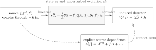
Kubo response separates the source $f$, coupled operator $B$, and measured observable $A$. The retarded commutator gives the state-mediated response. If $A$ depends explicitly on the source, its derivative contributes an additional instantaneous contact term.

General Space-Time Form

Let the source have components $f_b(\mathbf r,t)$ and write

$$H_{\mathrm{pert}}(t) = -\sum_b \int d^d r\, f_b(\mathbf r,t) B_b(\mathbf r).$$

The induced change in $A_a(\mathbf r,t)$ is

$$\begin{aligned} \delta\langle A_a(\mathbf r,t) \rangle ={}& \sum_b \int_{-\infty}^{\infty} dt' \int d^d r' \\ &\times \chi^R_{ab} (\mathbf r,t;\mathbf r',t') f_b(\mathbf r',t'). \end{aligned}$$

The retarded kernel is

$$\begin{aligned} \chi^R_{ab} (\mathbf r,t;\mathbf r',t') ={}& \frac{i}{\hbar} \theta(t-t') \\ &\times \left\langle \left[ A_{a,H}(\mathbf r,t), B_{b,H}(\mathbf r',t') \right] \right\rangle_0. \end{aligned}$$

On a lattice, replace the spatial integrals by site sums. The formula remains valid for a nonstationary reference state, but the kernel then depends on $t$ and $t'$ separately.

Derivation from the Density Operator

Write

$$H(t) = H_0+\lambda H_{\mathrm{pert}}(t),$$

where $\lambda$ tracks source order. In the interaction picture,

$$i\hbar \frac{d\rho_I}{dt} = \lambda [H_{\mathrm{pert},I}(t),\rho_I(t)].$$

To first order, replace $\rho_I(t)$ on the right by the unperturbed state $\rho_0$:

$$\begin{aligned} \rho_I(t) ={}& \rho_0 - \frac{i\lambda}{\hbar} \int_{t_0}^{t} dt'\, [H_{\mathrm{pert},I}(t'),\rho_0] \\ &+ O(\lambda^2). \end{aligned}$$

For $H_{\mathrm{pert},I}(t')=-f(t')B_I(t')$,

$$\begin{aligned} \delta\rho_I(t) ={}& \frac{i\lambda}{\hbar} \int_{t_0}^{t} dt'\, f(t') [B_I(t'),\rho_0] \\ &+ O(\lambda^2). \end{aligned}$$

Taking the trace with $A_I(t)$ and using cyclicity,

$$\begin{aligned} \delta\langle A(t)\rangle ={}& \frac{i\lambda}{\hbar} \int_{t_0}^{t} dt'\, f(t') \\ &\times \left\langle [A_I(t),B_I(t')] \right\rangle_0 + O(\lambda^2). \end{aligned}$$

Extending the integral over all $t'$ inserts $\theta(t-t')$. Setting $\lambda=1$ after identifying the first-order coefficient gives the Kubo formula.

The derivation assumes that the initial state is unmodified at the lower integration limit. Adiabatic switching from the distant past, a finite preparation time, and a quench protocol are physically different prescriptions and can select different steady or transient responses.

Functional-Derivative Definition

Operationally,

$$\chi^R_{AB}(t,t') = \left. \frac{ \delta\langle A(t)\rangle_f }{ \delta f(t') } \right|_{f=0}$$

when $A$ has no explicit source dependence. This definition makes clear that a susceptibility has units of detector divided by source.

For multiple components,

$$\chi^R_{ab} = \left. \frac{ \delta\langle A_a\rangle_f }{ \delta f_b } \right|_{f=0}.$$

The response can be anisotropic, nonlocal, and nondiagonal in internal indices even when the source is scalar.

Stationarity and Translation Invariance

Suppose

$$[H_0,\rho_0] = 0.$$

Then the reference state is stationary and

$$\chi^R_{AB}(t,t') = \chi^R_{AB}(t-t').$$

If the Hamiltonian, state, and geometry are also translation invariant,

$$\chi^R_{ab} (\mathbf r,t;\mathbf r',t') = \chi^R_{ab} (\mathbf r-\mathbf r',t-t').$$

Use the Fourier convention

$$X(\mathbf q,\omega) = \int_{-\infty}^{\infty} dt \int d^d r\, e^{i\omega t-i\mathbf q\cdot\mathbf r} X(\mathbf r,t).$$

The convolution becomes

$$\delta\langle A_a(\mathbf q,\omega) \rangle = \sum_b \chi^R_{ab}(\mathbf q,\omega) f_b(\mathbf q,\omega).$$

With this $e^{+i\omega t}$ transform, a retarded function is analytic for $\operatorname{Im}\omega\gt0$. The retarded boundary value carries $+i0$ in denominators.

Lehmann Representation

Choose a common eigenbasis of $H_0$ and a stationary $\rho_0$:

$$H_0\lvert n\rangle = E_n\lvert n\rangle, \qquad \rho_0 = \sum_n p_n \lvert n\rangle\langle n\rvert.$$

Define

$$A_{nm} = \langle n\lvert A\rvert m\rangle, \qquad B_{mn} = \langle m\lvert B\rvert n\rangle.$$

The frequency-domain susceptibility is

$$\chi^R_{AB}(\omega) = \sum_{n,m} \frac{ (p_m-p_n) A_{nm}B_{mn} }{ \hbar\omega + E_n-E_m + i0 }.$$

This formula exposes four independent ingredients:

1. transition energies $E_m-E_n$;
2. source matrix elements $B_{mn}$;
3. detector matrix elements $A_{nm}$;
4. population differences $p_n-p_m$.

A pole in the spectrum is invisible if either the source or detector matrix element vanishes. Population differences encode absorption minus stimulated emission. In an inverted state they can reverse the sign of the absorptive response.

The infinitesimal $i0$ enforces the retarded boundary condition. Replacing it by a finite $\Gamma$ is a physical or phenomenological broadening assumption and must be justified separately.

Absorptive Response

For a Hermitian operator $A=B$,

$$\begin{aligned} \operatorname{Im} \chi^R_{AA}(\omega) ={}& \frac{\pi}{\hbar} \sum_{n,m} (p_n-p_m) \lvert A_{nm}\rvert^2 \\ &\times \delta\!\left( \omega-\frac{E_m-E_n}{\hbar} \right). \end{aligned}$$

For a thermal state and $\omega\gt0$, upward transitions have $p_n\gt p_m$, so this convention gives

$$\operatorname{Im} \chi^R_{AA}(\omega) \ge 0.$$

Let a real harmonic source be

$$f(t) = \operatorname{Re} \left[ f_0e^{-i\omega t} \right].$$

The cycle-averaged work done on the system is

$$\overline P = \frac{\omega}{2} \lvert f_0\rvert^2 \operatorname{Im} \chi^R_{BB}(\omega)$$

for the coupling $H_{\mathrm{pert}}=-fB$. The imaginary part is therefore the absorptive or dissipative component under these conventions. The real part is reactive: it changes the in-phase response and stores rather than irreversibly absorbs energy over a cycle.

This positivity statement applies to a passive equilibrium state and a diagonal source–detector choice. A generic cross-susceptibility need not have a sign-definite imaginary part.

Causality and Dispersion Relations

Because

$$\chi^R_{AB}(t) = 0 \qquad \text{for }t\lt0,$$

its Fourier transform is analytic in the upper half-plane. Under suitable decay or subtraction conditions,

$$\operatorname{Re} \chi^R_{AB}(\omega) = \frac{1}{\pi} \operatorname{PV} \int_{-\infty}^{\infty} d\omega'\, \frac{ \operatorname{Im}\chi^R_{AB}(\omega') }{ \omega'-\omega }.$$

A companion relation reconstructs the imaginary part from the real part. These Kramers–Kronig relations follow from causality and analyticity, not from a particular microscopic model.

Slow high-frequency decay may require subtracted dispersion relations. Truncating a measured frequency interval can also make a direct numerical transform unreliable.

Static Response Is Not One Limit

Several quantities are casually called “the static susceptibility”:

• the thermodynamic derivative after the system re-equilibrates;
• $\chi^R(\mathbf q,\omega=0)$ at finite $\mathbf q$;
• the limit $\omega\to0$ after the thermodynamic limit;
• the uniform limit $\mathbf q\to0$;
• the response of an isolated finite system under adiabatic switching.

They need not agree.

For an equilibrium Hamiltonian

$$H_f = H_0-fB,$$

the isothermal susceptibility is

$$\chi_T^{BB} = \left. \frac{\partial\langle B\rangle_f} {\partial f} \right|_{f=0}.$$

In a canonical ensemble it can be written

$$\chi_T^{BB} = \int_0^\beta d\lambda\, \left\langle \delta B(-i\hbar\lambda) \delta B(0) \right\rangle_\beta,$$

where

$$B(-i\hbar\lambda) = e^{\lambda H_0} B e^{-\lambda H_0}.$$

If $[B,H_0]=0$, this reduces to

$$\chi_T^{BB} = \beta \left( \langle B^2\rangle_\beta - \langle B\rangle_\beta^2 \right).$$

Fluctuations and Susceptibilities develops this equilibrium identity, the general Kubo–Mori covariance, and the energy, number, and magnetization applications. The present page keeps the real-time retarded response and order-of-limits analysis as its canonical subject.

Yet the isolated retarded self-response of a conserved $B$ is zero because $[B(t),B]=0$. Re-equilibration changes the statistical weights of conserved sectors; closed-system unitary response cannot do so by itself. This distinction is essential for uniform magnetization, total particle number, and other conserved quantities.

Order of Limits

For a spatial response $\chi(\mathbf q,\omega)$, compare

$$\chi_{\mathrm{static}} = \lim_{\mathbf q\to0} \lim_{\omega\to0} \chi(\mathbf q,\omega)$$

with

$$\chi_{\mathrm{uniform}} = \lim_{\omega\to0} \lim_{\mathbf q\to0} \chi(\mathbf q,\omega).$$

The first lets an arbitrarily slowly varying spatial perturbation equilibrate before making it uniform. The second makes the perturbation uniform first, so conservation laws can block relaxation. Hydrodynamic poles often make the limits noncommuting.

Transport adds further limits:

$$L\to\infty, \qquad \omega\to0, \qquad \mathbf q\to0, \qquad \eta\to0^+.$$

A defensible result states their order. Taking $\omega\to0$ in a finite isolated spectrum generally produces delta functions or zero response rather than a bulk dc coefficient.

Explicit Source Dependence and Contact Terms

The commutator formula is not always the whole derivative. Suppose the measured operator itself depends on the source:

$$A[f] = A^{(0)} + fD + O(f^2).$$

Then

$$\begin{aligned} \delta\langle A(t)\rangle ={}& \int dt'\, \chi^R_{A^{(0)}B}(t,t') f(t') \\ &+ \langle D\rangle_0 f(t). \end{aligned}$$

Equivalently, the full response kernel contains

$$K_{AB}(t,t') = \chi^R_{A^{(0)}B}(t,t') + \langle D\rangle_0 \delta(t-t').$$

The instantaneous term is often called a contact, diamagnetic, or seagull term depending on context. Omitting it can violate gauge invariance, conservation-law sum rules, or the correct static limit.

If $A[f]$ is defined as a derivative of the Hamiltonian, the contact term comes from a second source derivative of $H[f]$. Its sign must be derived from that definition rather than memorized.

Magnetic Susceptibility

Let a field in energy units couple to local spins:

$$H_{\mathrm{pert}}(t) = -\sum_{j,\beta} h_j^\beta(t) s_j^\beta.$$

The response is

$$\begin{aligned} \delta\langle s_i^\alpha(t) \rangle ={}& \sum_{j,\beta} \int dt'\, \\ &\times \chi^R_{s_i^\alpha s_j^\beta}(t,t') h_j^\beta(t'). \end{aligned}$$

For a homogeneous system, Fourier transformation gives a tensor

$$\chi_{\alpha\beta}^R(\mathbf q,\omega).$$

The uniform static susceptibility is related to derivatives of total magnetization after specifying equilibration and volume normalization. If $M^z$ is conserved,

$$\chi_{M^zM^z}^R(\mathbf q=0,\omega) = 0$$

for the isolated commutator response, while the equilibrium isothermal susceptibility can be

$$\chi_T = \frac{\beta}{V} \left[ \langle(M^z)^2\rangle - \langle M^z\rangle^2 \right].$$

There is no contradiction: these quantities implement different protocols.

Density Response and Compressibility

Use a local chemical-potential source,

$$H_{\mathrm{pert}}(t) = -\int d^d r\, \delta\mu(\mathbf r,t) n(\mathbf r).$$

Then

$$\delta\langle n(\mathbf q,\omega) \rangle = \chi_{nn}^R(\mathbf q,\omega) \delta\mu(\mathbf q,\omega).$$

The equilibrium compressibility probes a static, long-wavelength density response. Two common conventions are

$$\kappa_n = \frac{\partial n}{\partial\mu}$$

and

$$\kappa_T = \frac{1}{n^2} \frac{\partial n}{\partial\mu}.$$

They differ by $n^{-2}$, so the symbol $\kappa$ is incomplete without a definition.

At exactly $\mathbf q=0$, the density operator is total particle number. If it is conserved, its finite-frequency retarded self-response vanishes. The thermodynamic compressibility instead compares equilibrium states with different chemical-potential weights. The static and uniform limits must therefore be distinguished.

Electrical Conductivity

Conductivity is the standard example in which a contact term is indispensable. For particles of charge $q$ in a spatially uniform vector potential,

$$H[\mathbf A] = \sum_{i=1}^{N} \frac{ \left( \mathbf p_i-q\mathbf A \right)^2 }{2m} + V.$$

Expanding to second order,

$$H[\mathbf A] = H_0 - \mathbf A\cdot\mathbf J^p + \frac{Nq^2}{2m} \mathbf A^2,$$

where $\mathbf J^p$ is the total paramagnetic current. The physical current density is

$$\mathbf j[\mathbf A] = -\frac{1}{V} \frac{\partial H}{\partial\mathbf A} = \mathbf j^p - \frac{nq^2}{m} \mathbf A.$$

Define the paramagnetic current-response tensor per volume,

$$\Pi_{\alpha\beta}^R(\omega) = \frac{1}{V} \chi^R_{J_\alpha^pJ_\beta^p}(\omega),$$

and the diamagnetic tensor

$$D_{\alpha\beta} = \frac{nq^2}{m} \delta_{\alpha\beta}.$$

Then

$$\delta j_\alpha(\omega) = \sum_\beta \left[ \Pi_{\alpha\beta}^R(\omega) - D_{\alpha\beta} \right] A_\beta(\omega).$$

With vanishing scalar potential and the Fourier convention used here,

$$E_\beta(\omega) = i\omega A_\beta(\omega).$$

The optical conductivity is therefore

$$\sigma_{\alpha\beta}(\omega) = \frac{i}{\omega+i0} \left[ D_{\alpha\beta} - \Pi_{\alpha\beta}^R(\omega) \right].$$

The signs follow from three stated choices: charge enters as $\mathbf p-q\mathbf A$, current is $-\partial H/\partial\mathbf A$, and Fourier transforms use $e^{+i\omega t}$. Other conventions can rearrange signs while leaving measurable response unchanged.

On a lattice, $D_{\alpha\beta}$ is an expectation of the appropriate kinetic-energy or stress tensor rather than simply $nq^2/m$. It must be derived by coupling the lattice Hamiltonian to a gauge field, usually through Peierls phases.

Drude and regular weight

A common decomposition is

$$\operatorname{Re} \sigma(\omega) = \pi D_{\mathrm{Dr}} \delta(\omega) + \sigma_{\mathrm{reg}}(\omega).$$

$D_{\mathrm{Dr}}\gt0$ signals a ballistic zero-frequency contribution under the stated order of limits. It is not the same symbol as the bare diamagnetic tensor before paramagnetic cancellation.

For a clean noninteracting continuum with conserved total momentum,

$$\Pi^R(\omega) = 0$$

at zero wavevector, giving

$$\sigma(\omega) = \frac{i}{\omega+i0} \frac{nq^2}{m}.$$

Its real part is a delta function, not a finite dc conductivity. A finite resistivity requires a mechanism that relaxes the relevant current or momentum, such as disorder, a lattice with suitable scattering, umklapp processes, phonons, boundaries, or coupling to other degrees of freedom.

Gauge and Conservation Checks

Electromagnetic response must be gauge consistent. A scalar potential and a longitudinal vector potential can represent the same electric field after a gauge transformation. Density and current correlators are therefore linked by the continuity equation and associated Ward identities.

Practical checks include:

• include both paramagnetic and contact contributions;
• use a current operator derived from the same gauged Hamiltonian;
• verify charge conservation and the continuity equation;
• check the optical identities developed on Sum Rules;
• distinguish a uniform vector potential that is pure gauge from flux through a periodic ring;
• state whether the thermodynamic limit is taken before removing the vector potential or frequency regulator.

A violation often signals a missing contact term, inconsistent truncation, nonconserving approximation, or incompatible boundary convention.

Finite Systems and Numerical Spectra

For a finite isolated system, the Lehmann representation consists of discrete poles. Its absorptive part is a sum of delta functions:

$$\chi''(\omega) = \sum_\ell w_\ell \delta(\omega-\omega_\ell).$$

Replacing each delta function by

$$\delta_\eta(\omega-\omega_\ell) = \frac{1}{\pi} \frac{ \eta }{ (\omega-\omega_\ell)^2+\eta^2 }$$

is a plotting or regularization choice unless $\eta$ is derived from a physical decay process. Report it explicitly.

For bulk response:

1. resolve exact symmetry sectors and matrix elements;
2. include contact terms and conserved contributions;
3. check sum rules at every size;
4. vary the broadening independently of system size;
5. take a controlled thermodynamic limit;
6. only then analyze zero-frequency or long-time behavior.

A smooth curve from one broadened cluster is not evidence for a finite lifetime or dc transport coefficient.

Imaginary-Time Calculations

Equilibrium Monte Carlo and Matsubara methods often compute an imaginary-time correlator rather than $\chi^R(\omega)$ directly. The two share spectral information, but obtaining real-frequency response requires analytic continuation.

That inverse problem is ill-conditioned: many real-frequency spectra can fit noisy imaginary-time data within error bars. A trustworthy continuation reports priors, regularization, covariance of the input data, resolution limits, and tests on synthetic spectra.

The Kubo formula does not make analytic continuation automatic. It identifies the target retarded object; a separate inference problem remains.

Analytic Continuation develops that inference problem, including covariance, channel-valid constraints, static terms, method limitations, and feature-level resolution.

Validity of Linear Response

The response expansion requires the induced change to remain first order over the observation window. It can fail when:

• the source is not small relative to intrinsic scales;
• a resonant drive acts long enough for secular growth or saturation;
• the source changes populations appreciably;
• the system crosses a phase boundary;
• heating changes the reference state;
• nonlinear selection rules or harmonics are the observable of interest;
• the background is strongly driven and not stationary.

A small instantaneous amplitude does not guarantee linear behavior for arbitrarily long time. Near a narrow resonance, a dimensionless accumulated transition amplitude can become order one.

For a periodically driven or aging reference state, use a two-time or Floquet response kernel rather than importing a one-frequency equilibrium susceptibility.

Calculation Workflow

1. Write $H_{\mathrm{pert}}$ with its sign and source units.
2. Identify the coupled operator $B$ and detector $A$.
3. Specify $\rho_0$, temperature, chemical potential, and stationarity.
4. State spatial, temporal, Fourier, and volume normalizations.
5. Derive any explicit source dependence of $A$.
6. Use symmetry and conservation laws before evaluating matrix elements.
7. Compute the retarded commutator or its Lehmann representation.
8. Add contact terms before imposing gauge or static limits.
9. State the order of $L$, $\mathbf q$, $\omega$, and $\eta$ limits.
10. Check causality, Kramers–Kronig relations, positivity where applicable, and exact sum rules.
11. Test that the induced response remains small.
12. Separate intrinsic linewidths from finite-time, finite-size, and numerical broadening.

Common Mistakes

• Writing $\chi^R$ without stating whether the perturbation is $-fB$ or $+fB$.
• Swapping source and detector labels in a cross-susceptibility.
• Using the retarded Green-function sign while calling the result the susceptibility defined here.
• Omitting $\theta(t-t')$ or the retarded $+i0$ prescription.
• Assuming every linear-response calculation requires thermal equilibrium.
• Applying an equilibrium fluctuation–dissipation relation to a nonstationary state.
• Identifying $\chi^R(\omega=0)$ with a thermodynamic derivative without checking equilibration and conserved quantities.
• Taking $\mathbf q\to0$ and $\omega\to0$ without specifying their order.
• Omitting the diamagnetic or other contact term in conductivity.
• Using a current operator inconsistent with the gauged Hamiltonian.
• Interpreting $i0$ as a physical linewidth.
• Interpreting chosen Lorentzian broadening as intrinsic decay.
• Reading a finite dc coefficient from a finite isolated cluster.
• Assuming interactions alone guarantee current relaxation when momentum remains conserved.
• Trusting linear response near resonance after the induced change becomes order one.

Exercises

Sign of the retarded kernel

Starting from the interaction-picture density operator, derive the sign of $\chi^R_{AB}$ for

$$H_{\mathrm{pert}}(t) = -f(t)B.$$

How does the result change for $H_{\mathrm{pert}}=+fB$?

Solution

To first order,

$$\delta\rho_I(t) = -\frac{i}{\hbar} \int_{t_0}^{t} dt'\, [H_{\mathrm{pert},I}(t'),\rho_0].$$

Substitution gives

$$\delta\rho_I(t) = \frac{i}{\hbar} \int_{t_0}^{t} dt'\, f(t') [B_I(t'),\rho_0].$$

Therefore

$$\begin{aligned} \delta\langle A(t)\rangle &= \operatorname{Tr} \left[ \delta\rho_I(t)A_I(t) \right] \\ &= \frac{i}{\hbar} \int_{t_0}^{t} dt'\, f(t') \langle[A_I(t),B_I(t')]\rangle_0. \end{aligned}$$

Thus

$$\chi^R_{AB}(t,t') = \frac{i}{\hbar} \theta(t-t') \langle[A_H(t),B_H(t')]\rangle_0.$$

Changing the perturbation to $+fB$ reverses the overall sign.

Lehmann weights and absorption

For a thermal state and Hermitian $A$, show that

$$\operatorname{Im} \chi^R_{AA}(\omega) \ge 0$$

for $\omega\gt0$ under this page’s conventions.

Solution

At positive frequency, the delta function selects

$$E_m-E_n = \hbar\omega \gt 0.$$

Thermal probabilities obey

$$p_n = \frac{e^{-\beta E_n}}{Z} \gt \frac{e^{-\beta E_m}}{Z} = p_m.$$

Every selected term in

$$\operatorname{Im} \chi^R_{AA}(\omega) = \frac{\pi}{\hbar} \sum_{n,m} (p_n-p_m) \lvert A_{nm}\rvert^2 \delta(\omega-\omega_{mn})$$

is therefore nonnegative. This is the spectral origin of positive absorbed power for a passive thermal state.

Transverse spin susceptibility

Let

$$H_0 = \frac{\hbar\Omega}{2} \sigma_z, \qquad H_{\mathrm{pert}} = -f(t)\sigma_x.$$

For a thermal state, compute $\chi^R_{xx}(t)$ and $\chi^R_{xx}(0)$ in frequency space.

Solution

The Heisenberg operator is

$$\sigma_x(t) = \sigma_x\cos(\Omega t) - \sigma_y\sin(\Omega t).$$

Hence

$$[\sigma_x(t),\sigma_x] = 2i\sigma_z \sin(\Omega t).$$

The thermal polarization is

$$\langle\sigma_z\rangle_\beta = -\tanh\!\left( \frac{\beta\hbar\Omega}{2} \right).$$

Therefore

$$\chi^R_{xx}(t) = \frac{2}{\hbar} \tanh\!\left( \frac{\beta\hbar\Omega}{2} \right) \theta(t) \sin(\Omega t).$$

Fourier transformation gives

$$\chi^R_{xx}(\omega) = \frac{ 2\Omega }{ \hbar \left[ \Omega^2-(\omega+i0)^2 \right] } \tanh\!\left( \frac{\beta\hbar\Omega}{2} \right).$$

Thus

$$\chi^R_{xx}(0) = \frac{2}{\hbar\Omega} \tanh\!\left( \frac{\beta\hbar\Omega}{2} \right).$$

This agrees with the small static tilt of the equilibrium spin.

Conserved quantity paradox

Suppose $[B,H_0]=0$. Show that the isolated retarded self-response $\chi^R_{BB}(t)$ vanishes, while the canonical isothermal susceptibility can be $\beta\operatorname{Var}(B)$.

Solution

Conservation gives

$$B_H(t) = B.$$

Therefore

$$[B_H(t),B] = 0$$

and

$$\chi^R_{BB}(t) = 0.$$

For the equilibrium Hamiltonian $H_f=H_0-fB$, commuting $B$ permits direct differentiation of the Boltzmann weights:

$$\left. \frac{\partial\langle B\rangle_f} {\partial f} \right|_{f=0} = \beta \left( \langle B^2\rangle - \langle B\rangle^2 \right).$$

The thermodynamic protocol reweights sectors with different $B$ after equilibration. The isolated unitary protocol preserves their populations. The two susceptibilities answer different physical questions.

Diamagnetic term for free particles

For

$$H[\mathbf A] = \sum_i \frac{ (\mathbf p_i-q\mathbf A)^2 }{2m},$$

derive the physical current and the zero-wavevector conductivity when the total paramagnetic current commutes with $H_0$.

Solution

Differentiating the Hamiltonian,

$$\mathbf j = -\frac{1}{V} \frac{\partial H}{\partial\mathbf A} = \frac{q}{mV} \sum_i\mathbf p_i - \frac{nq^2}{m} \mathbf A.$$

The first term is $\mathbf j^p$. Because total momentum is conserved,

$$\Pi^R(\omega) = 0$$

at zero wavevector. Hence

$$\sigma(\omega) = \frac{i}{\omega+i0} \frac{nq^2}{m}.$$

Using

$$\frac{i}{\omega+i0} = i\operatorname{PV} \frac{1}{\omega} + \pi\delta(\omega),$$

gives

$$\operatorname{Re}\sigma(\omega) = \pi \frac{nq^2}{m} \delta(\omega).$$

The contact term produces ballistic Drude weight. Dropping it would incorrectly give zero electromagnetic response.

Static and uniform density limits

Explain why

$$\lim_{\mathbf q\to0} \lim_{\omega\to0} \chi_{nn}^R(\mathbf q,\omega)$$

can differ from

$$\lim_{\omega\to0} \lim_{\mathbf q\to0} \chi_{nn}^R(\mathbf q,\omega).$$

Solution

At nonzero but small $\mathbf q$, density can redistribute over long distances. Taking $\omega\to0$ first allows the spatial modulation to equilibrate; sending $\mathbf q\to0$ afterward probes compressibility.

Taking $\mathbf q\to0$ first turns the density operator into total particle number. If total number is conserved, its finite-frequency retarded self-response vanishes. The subsequent $\omega\to0$ limit remains constrained by that conservation law.

The two orders describe different protocols, so their disagreement is physical rather than an algebraic inconsistency.

Cross-Links

• How Quantum Matter Is Measured places linear response inside the larger chain from a controlled source and detector record to a calibrated material inference.
• Terahertz and Infrared Probes connects measured power or electric-field waveforms to the complex conductivity defined here.
• Transport Measurements connects terminal wiring, low-frequency protocols, geometry, tensor inversion, and sweep history to the conductivity limits defined here.
• Linear Response Formula Sheet provides the compact convention, spectral, static-limit, contact-term, and transport lookup.
• Correlation Functions Overview
• Structure Factors
• Green Functions in Many-Body QM
• Retarded and Advanced Response
• Susceptibilities
• Fluctuation–Dissipation Theorem
• Sum Rules
• Transport Coefficients Preview
• Chern Numbers in Band Theory specializes the clean transverse Kubo response to occupied Bloch bands and derives the TKNN integer.
• Weak Localization specializes conductivity response to disorder-averaged diffusive interference and identifies the Cooperon correction measured in low fields.
• Thermal Density Operators
• Canonical Ensemble
• Grand-Canonical Ensemble
• Hubbard Model
• Heisenberg Model
• Green Functions and Response Preview
• Retarded and Advanced Green Functions
• Spectral Representation of Green Functions
• Interaction Picture
• Linear Response Preview
• First-Order Transition Probability
• Fluctuation–Dissipation Relation
• Noise Spectra
• Fourier-Transform Conventions
• Correlation-Functions Formula Card

References

1. R. Kubo, “Statistical-Mechanical Theory of Irreversible Processes. I”, Journal of the Physical Society of Japan 12, 570–586 (1957).
2. H. B. Callen and T. A. Welton, “Irreversibility and Generalized Noise”, Physical Review 83, 34–40 (1951).
3. R. Kubo, “The Fluctuation-Dissipation Theorem”, Reports on Progress in Physics 29, 255–284 (1966).
4. W. Kohn, “Theory of the Insulating State”, Physical Review 133, A171–A181 (1964).
5. J. M. Luttinger, “Theory of Thermal Transport Coefficients”, Physical Review 135, A1505–A1514 (1964).
6. D. J. Scalapino, S. R. White, and S. C. Zhang, “Insulator, Metal, or Superconductor: The Criteria”, Physical Review B 47, 7995–8007 (1993).
7. G. D. Mahan, Many-Particle Physics, 3rd ed., Springer (2000).
8. A. L. Fetter and J. D. Walecka, Quantum Theory of Many-Particle Systems, Dover (2003).
9. G. F. Giuliani and G. Vignale, Quantum Theory of the Electron Liquid, Cambridge University Press (2005).
10. A. Altland and B. Simons, Condensed Matter Field Theory, 2nd ed., Cambridge University Press (2010).