Connected Correlation Functions

A connected correlation function removes every contribution that factorizes into lower-order expectation values. At second order and in a fixed operator order,

$$\left\langle AB \right\rangle_c = \left\langle AB \right\rangle - \left\langle A\right\rangle \left\langle B\right\rangle.$$

Equivalently, with centered operators

$$\delta A = A-\langle A\rangle I, \qquad \delta B = B-\langle B\rangle I,$$

one has

$$\left\langle AB \right\rangle_c = \left\langle \delta A\,\delta B \right\rangle.$$

The subtraction isolates joint fluctuations not explained by the one-point profiles. Spatially, it is the object that clusters in a pure short-range-correlated phase. Combinatorially, its higher-order generalizations are cumulants. Diagrammatically, connected pieces are selected by the logarithm of a generating functional.

Connected does not mean symmetrized, entangled, interacting, irreducible, amputated, or causal. Each of those words performs a different operation.

Canonical Scope

This page is the canonical home for connected correlation functions in many-body quantum mechanics. It owns:

• ordered two-point and higher connected cumulants;
• moment–cumulant relations and logarithmic generating functions;
• distinctions from covariance, entanglement, interaction, and response;
• cluster decomposition and the role of pure phases;
• how connected subtraction behaves in exponentially clustering, algebraic, and ordered regimes;
• exponential, effective, and second-moment correlation lengths;
• global constraints, ensemble effects, and finite-size tails;
• numerical, experimental, and statistical subtraction practices.

Neighboring canonical pages retain related material:

• Correlations and Covariance owns real symmetrized covariance for quantum observables.
• Marginals and Correlations owns product-state reconstruction from complete local operator data and the distinction between total and entangled correlation.
• Equal-Time Correlations owns static spin, density, one-body, and pair operator choices.
• Long-Range Order owns nonzero correlation limits, squared-order criteria, and extensive peak scaling.
• Time-Dependent Correlations owns unequal-time ordering, Lehmann spectra, recurrence, and dynamical plateaus.
• Sources and Generating Functionals in QM owns path-integral source differentiation.
• Diagrammatic Methods Preview owns connected diagrams, self-energies, and diagrammatic reducibility.
• Later pages in this chapter own structure-factor Fourier conventions, susceptibilities, and sum rules.

Convention Ledger

Unless stated otherwise:

1. $\langle X\rangle=\operatorname{Tr}(\rho X)$.
2. Every operator product keeps its written order.
3. A superscript or subscript $c$ denotes the connected cumulant for that same ordering prescription.
4. Local operators have bounded support unless a continuum or extensive observable is stated.
5. Spatial distance is measured between operator supports, not merely coordinate labels.
6. Correlation lengths refer to connected correlators.
7. Thermodynamic and large-distance limits are stated explicitly.
8. A finite lattice has $L$ sites and linear size $\ell$ when both are needed.

For noncommuting operators, different orderings define different moments and therefore different cumulants. Subtracting disconnected pieces never authorizes reordering.

Two-Point Connected Function

For insertions labeled by position, time, component, or mode,

$$\begin{aligned} G_{AB}^c(1,2) &= \left\langle A(1)B(2) \right\rangle_c \\ &= \left\langle A(1)B(2) \right\rangle - \left\langle A(1) \right\rangle \left\langle B(2) \right\rangle. \end{aligned}$$

The disconnected product is what this particular second moment would contain if the two insertions factorized:

$$G_{AB}^{\mathrm{disc}}(1,2) = \left\langle A(1)\right\rangle \left\langle B(2)\right\rangle.$$

Thus

$$G_{AB} = G_{AB}^{\mathrm{disc}} + G_{AB}^c.$$

This is an algebraic identity, not an approximation.

Complex ordered values

For Hermitian $A$ and $B$,

$$\left\langle AB \right\rangle_c^* = \left\langle BA \right\rangle_c.$$

An ordered connected correlator may be complex. Its symmetrized real part is

$$\operatorname{Cov}(A,B) = \frac{1}{2} \left\langle \delta A\,\delta B + \delta B\,\delta A \right\rangle.$$

Connected subtraction changes means; symmetrization changes order. Correlations and Covariance owns the latter as a measurement statistic.

Higher Connected Functions

At third order,

$$\begin{aligned} \langle ABC\rangle_c ={}& \langle ABC\rangle - \langle A\rangle\langle BC\rangle - \langle B\rangle\langle AC\rangle \\ &- \langle C\rangle\langle AB\rangle + 2 \langle A\rangle \langle B\rangle \langle C\rangle. \end{aligned}$$

The operator order inside each moment is inherited from the declared prescription. For example, $\langle AC\rangle$ retains $A$ before $C$.

If every one-point function vanishes, the fourth connected function is

$$\begin{aligned} \langle ABCD\rangle_c ={}& \langle ABCD\rangle - \langle AB\rangle \langle CD\rangle \\ &- \langle AC\rangle \langle BD\rangle - \langle AD\rangle \langle BC\rangle. \end{aligned}$$

For nonzero means, additional partitions containing singleton blocks must be included.

General partition formula

Let $\Pi_n$ be the set of partitions of $\{1,\ldots,n\}$. For a specified source and ordering convention,

$$\begin{aligned} \left\langle X_1\cdots X_n \right\rangle_c ={}& \sum_{\pi\in\Pi_n} \left( \lvert\pi\rvert-1 \right)! (-1)^{\lvert\pi\rvert-1} \\ &\times \prod_{B\in\pi} \left\langle \prod_{i\in B}^{\mathrm{ord}} X_i \right\rangle. \end{aligned}$$

The inner product follows the inherited order within the block. The outer factors are ordinary complex numbers and commute. For fermionic fields, contour-ordered objects, or generalized operator exponentials, signs and source types must follow the chosen generating convention rather than being guessed from the classical formula.

Generating Connected Cumulants

For commuting scalar sources $J_a$ and a declared ordered exponential, define

$$Z[J] = \left\langle \mathcal O \exp\!\left( \sum_a J_a X_a \right) \right\rangle,$$

where $\mathcal O$ denotes the ordering prescription. Normalize so that

$$Z[0] = 1.$$

The cumulant-generating functional is

$$W[J] = \log Z[J].$$

Then

$$\left. \frac{\partial^n W}{ \partial J_{a_1}\cdots\partial J_{a_n} } \right|_{J=0} = \left\langle X_{a_1}\cdots X_{a_n} \right\rangle_c$$

with the ordering and any convention-dependent factors fixed by the definition of $Z$.

The logarithm removes products of independent pieces because

$$Z_{A\cup B} = Z_A Z_B$$

for factorized sectors, while

$$\log Z_{A\cup B} = \log Z_A + \log Z_B.$$

Mixed derivatives between independent sectors therefore vanish.

Connected is not the same as one-particle irreducible. A connected function may still separate after cutting one internal line. Legendre transformation, amputation, and one-particle irreducibility are later operations.

Gaussian States and Wick Factorization

For observables linear in the canonical fields of a Gaussian state, with a specified ordering prescription, all connected cumulants above second order vanish:

$$\left\langle X_1\cdots X_n \right\rangle_c = 0, \qquad n>2.$$

At fourth order with zero means,

$$\begin{aligned} \langle ABCD\rangle ={}& \langle AB\rangle \langle CD\rangle + \langle AC\rangle \langle BD\rangle \\ &+ \langle AD\rangle \langle BC\rangle \end{aligned}$$

for commuting Gaussian variables or bosonic fields in a compatible ordering. Fermionic Wick contractions carry permutation signs. Substituting the Wick sum into the fourth-cumulant formula gives zero.

The restriction to linear fields matters: nonlinear observables such as a squared Gaussian field generally have nonzero higher cumulants. Conversely, vanishing of one measured fourth cumulant does not prove that a state is Gaussian. Gaussianity requires the full hierarchy of higher connected functions of the canonical fields to vanish in the relevant ordering.

Interactions often generate non-Gaussian connected cumulants, but “interacting” and “non-Gaussian” are not synonyms. Quadratic effective theories can describe interacting systems approximately, while a noninteracting Hamiltonian with a non-Gaussian initial state can have nonzero higher cumulants.

Connected Is Not Entangled

If two regions are in a product state,

$$\rho_{XY} = \rho_X\otimes\rho_Y,$$

then for every local pair $A_X$ and $B_Y$,

$$\left\langle A_XB_Y \right\rangle_c = 0.$$

The converse is false for one selected pair. A state can be correlated in operators not tested by $A_X$ and $B_Y$.

Even a nonzero connected correlator does not prove entanglement. Consider

$$\rho_{\mathrm{cc}} = \frac{1}{2} \left( \lvert 00\rangle\langle00\rvert + \lvert 11\rangle\langle11\rvert \right).$$

This state is separable, yet

$$\langle Z_1\rangle = \langle Z_2\rangle = 0, \qquad \langle Z_1Z_2\rangle_c = 1.$$

The connected correlation is classical uncertainty about which aligned product state was prepared.

If factorization holds for complete operator bases on both regions,

$$\left\langle A_\mu B_\nu \right\rangle = \left\langle A_\mu\right\rangle \left\langle B_\nu\right\rangle$$

for all $\mu,\nu$, then the joint state is a product. That is a complete tomography statement, much stronger than checking one correlator. Marginals and Correlations owns this reconstruction boundary.

Connected Is Not Interaction

Connected correlations can arise without dynamical interactions:

• exchange statistics produces density antibunching or bunching;
• a fixed total charge produces compensating anticorrelation;
• a classically correlated mixture has nonzero connected moments;
• an initially entangled state can evolve under a noninteracting Hamiltonian;
• common external randomness can correlate otherwise uncoupled sectors.

Conversely, an interacting Hamiltonian does not guarantee a nonzero selected correlator. Symmetry can force it to vanish, a product mean-field approximation can set it to zero by construction, or the chosen operators can miss the correlated channel.

Connected correlation diagnoses failure of moment factorization for specified operators and a specified state. Its physical origin requires additional evidence.

Spatial Cluster Decomposition

Let $A_X$ and $B_Y$ be bounded local operators supported in regions $X$ and $Y$. A state clusters for this operator class if

$$\left\langle A_XB_Y \right\rangle_c \longrightarrow 0$$

as

$$\operatorname{dist}(X,Y) \longrightarrow \infty.$$

Cluster decomposition says that sufficiently distant bounded experiments become independent at the level of local moments. It is a property of the state, the operator class, and the limiting procedure. It is not guaranteed by writing down a local Hamiltonian.

Pure phases and mixtures

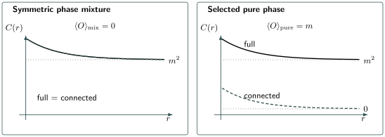
Phase selection changes what the subtraction removes. In a symmetric mixture, $\langle O\rangle=0$, so the connected correlator equals the full correlator and can retain the order plateau. In a selected pure phase, the full correlator approaches $m^2$ while subtraction leaves a connected fluctuation that clusters to zero.

Suppose a broken-symmetry pure phase has

$$\langle O_i\rangle = m.$$

Cluster decomposition gives

$$\langle O_iO_j\rangle \longrightarrow m^2,$$

while

$$\langle O_iO_j\rangle_c \longrightarrow 0.$$

Now form an equal mixture of two phases with order parameters $\pm m$. The mixture has

$$\langle O_i\rangle_{\mathrm{mix}} = 0$$

but can retain

$$\langle O_iO_j\rangle_{\mathrm{mix}} \longrightarrow m^2.$$

Therefore

$$\langle O_iO_j\rangle_{c,\mathrm{mix}} \longrightarrow m^2.$$

The mixture fails cluster decomposition because a global classical label, the selected phase, remains correlated across arbitrary distance.

A finite symmetry-preserving ground state can behave similarly over distances below the system size. It is incorrect to infer absence of order from a zero one-point function or to infer absence of a pure clustering phase from the finite-volume connected plateau. Spontaneous Symmetry Breaking owns the cat-state, source, tower-spectrum, and thermodynamic branch-selection mechanism.

Exponential Clustering

A short-range-correlated phase often satisfies

$$\left| \langle A_XB_Y\rangle_c \right| \leq C_{A,B} e^{-\operatorname{dist}(X,Y)/\xi}$$

at large separation, possibly with an algebraic prefactor.

For quantum lattice systems with sufficiently local bounded interactions, Lieb–Robinson locality and a suitable spectral gap imply exponential decay of ground-state connected correlations under precise hypotheses. The theorem’s correlation-length bound is controlled parametrically by a locality velocity divided by the gap, but it is not generally an equality for the physical correlation length. Area Laws separates this clustering theorem from the stronger entropy statement and records where the converse is rigorous.

Important qualifications include:

• ground-state degeneracy and phase-sector selection;
• operators that connect different ground sectors;
• long-range interactions;
• unbounded local degrees of freedom;
• gauge constraints and nonlocal observables;
• finite temperature and thermal phase transitions;
• topological sectors and boundary modes.

A spectral gap is a powerful sufficient ingredient in the local setting, not a universal one-line equivalence between “gapped” and “exponential” for every operator and geometry.

Correlation Lengths

There are several useful but inequivalent correlation lengths.

Asymptotic exponential length

For

$$C^c(r) \sim A \frac{ e^{-r/\xi} }{ r^p } \cos(Qr+\varphi),$$

$\xi$ is the exponential decay length. The amplitude, power $p$, oscillation wavevector $Q$, and phase $\varphi$ must be handled before fitting.

Several transfer-matrix eigenvalues or excitation channels can produce several lengths:

$$C^c(r) = \sum_a A_a e^{-r/\xi_a} \cos(Q_ar+\varphi_a) +\cdots.$$

The largest $\xi_a$ dominates only if its amplitude is nonzero in the chosen operator channel and the asymptotic regime is reached.

Effective local length

For a positive, nonoscillatory pure exponential sampled with spacing $a$,

$$\xi_{\mathrm{eff}}(r) = \frac{a}{ \log\!\left[ C^c(r)/C^c(r+a) \right] }.$$

A plateau of $\xi_{\mathrm{eff}}(r)$ can identify an asymptotic window. Sign changes, noise near zero, algebraic prefactors, multiple exponentials, and boundaries can make this estimator unstable or biased.

Second-moment length

For a periodic lattice and an ordering wavevector $\mathbf Q$, a common finite-size estimator is

$$\xi_2 = \frac{1}{ 2\sin(\lvert\mathbf q_{\min}\rvert/2) } \sqrt{ \frac{ S_c(\mathbf Q) }{ S_c(\mathbf Q+\mathbf q_{\min}) } -1 },$$

in lattice-spacing units. Here $S_c$ is the Fourier transform of the connected correlator and $\mathbf q_{\min}$ is the smallest compatible momentum increment.

This formula assumes a suitable Ornstein–Zernike-like small-momentum shape and geometry. Landau–Ginzburg Theory Preview derives the Gaussian kernel $r+c k^2$ and its pole length; the estimator here remains an operational definition rather than an assumption that the full system is Gaussian. Other boundary conditions, anisotropic systems, conserved constraints, and tensor channels require modified estimators. The second-moment length need not equal the asymptotic exponential length away from a scaling regime.

Structure Factors owns the Fourier normalization in depth; the formula appears here only to distinguish common definitions of $\xi$.

Algebraic and Critical Correlations

At a scale-invariant point or in a stable critical phase,

$$C_O^c(r) \sim \frac{ \cos(\mathbf Q\cdot\mathbf r+\varphi) }{ r^{2\Delta_O} },$$

where $\Delta_O$ is the scaling dimension of the operator channel.

There is no finite exponential correlation length at the critical point. Away from it, a scaling form is

$$C_O^c(r;\delta) = \frac{1}{ r^{2\Delta_O} } \mathcal F_\pm \left( \frac{r}{\xi} \right),$$

with

$$\xi \sim \lvert\delta\rvert^{-\nu}.$$

Here $\delta$ measures distance from criticality and the branches $\mathcal F_\pm$ can differ on the two sides.

Critical behavior requires several cautions:

• different operators have different scaling dimensions;
• symmetry can suppress the leading channel;
• dangerously irrelevant variables can modify naive finite-size scaling;
• logarithmic corrections can imitate drifting powers;
• anisotropic systems can have direction-dependent lengths;
• a quantum critical point includes temporal scaling and a dynamical exponent;
• a finite range of sizes can fit both a large finite $\xi$ and a power law.

Gaplessness does not force every correlator to decay algebraically, and one algebraic correlator does not determine the entire universality class.

Critical Exponents and Scaling owns the anomalous-dimension convention, Fisher relation, finite-size correction structure, and dynamic scaling that organize these critical correlators.

Long-Range Order and Connected Subtraction

Long-Range Order gives the canonical plateau, squared-order, and finite-size scaling criteria. Here the narrower question is what connected subtraction removes before and after phase selection.

For an order parameter $O_i$, a nonzero full plateau

$$\lim_{r\to\infty} \langle O_iO_{i+r}\rangle = m^2$$

is consistent with long-range order. In a selected clustering phase,

$$\langle O_i\rangle = m$$

and the connected plateau vanishes.

The connected correlator is therefore not always the best finite-volume detector of broken symmetry. In a symmetric finite state, subtracting zero leaves the full plateau, which is useful. In a selected phase, connected subtraction deliberately removes the order parameter and isolates fluctuations.

Always state which question is being asked:

• Does the phase possess order? Inspect full long-distance correlations or squared order parameters with finite-size scaling.
• Do fluctuations around a selected phase remain correlated? Inspect the connected function.
• Does a mixed state cluster? Inspect whether connected local correlations vanish after the thermodynamic and phase-selection prescription.

Global Constraints and Ensemble Tails

Let

$$N = \sum_j n_j$$

be exactly fixed. Then

$$\sum_j \langle \delta n_i\delta n_j \rangle = 0.$$

A positive onsite variance must be compensated by offsite anticorrelation. In a translation-invariant system of $L$ sites, this can produce a weak background of order $1/L$ spread across the sample.

Pointwise,

$$C_n^c(r) \longrightarrow 0$$

as $L\to\infty$ at fixed $r$ may coexist with an order-one integrated constraint:

$$\sum_r C_n^c(r) = 0.$$

This is why ensemble equivalence for local observables does not imply identical finite-size connected sums at zero momentum.

Similar tails arise from fixed magnetization, fixed energy, gauge constraints, and postselection. They are correlations induced by conditioning and conservation, not necessarily by a local force.

Extensive Observables and Cumulant Scaling

For an extensive observable

$$X = \sum_i x_i,$$

its variance is the sum of connected two-point functions:

$$\operatorname{Var}(X) = \sum_{i,j} \langle x_i x_j\rangle_c.$$

More generally,

$$\kappa_n(X) = \sum_{i_1,\ldots,i_n} \left\langle x_{i_1}\cdots x_{i_n} \right\rangle_c.$$

If the connected $n$-point function is absolutely summable in all relative coordinates, only tuples within a finite correlation volume contribute appreciably to each anchor point. Then

$$\kappa_n(X) \propto L$$

for an extensive sequence.

Near criticality or with long-range order, the correlation volume grows and cumulants can scale superextensively. Ratios such as Binder cumulants exploit this scaling, but their normalization and universal limits depend on geometry, boundary conditions, order-parameter symmetry, and ensemble.

The fluctuation and susceptibility consequences are developed in Fluctuations and Susceptibilities.

Inhomogeneous Profiles and Averaging Order

For an open, trapped, or disordered system, define the displacement-averaged connected correlator by subtracting local means before averaging:

$$\begin{aligned} \overline C_{AB}^c(r) ={}& \frac{1}{N_r} \sum_{i:\,i+r\in\Lambda} \big[ \langle A_iB_{i+r}\rangle \\ &\qquad- \langle A_i\rangle \langle B_{i+r}\rangle \big]. \end{aligned}$$

This generally differs from

$$\frac{1}{N_r} \sum_i \langle A_iB_{i+r}\rangle - \overline{\langle A\rangle} \, \overline{\langle B\rangle}.$$

The difference is the spatial covariance of the one-point profiles. Subtracting global means can mistake a trap shape, domain wall, density gradient, or disorder pattern for correlated fluctuations.

If disorder averaging is also performed, distinguish:

$$\overline{ \langle AB\rangle - \langle A\rangle\langle B\rangle }$$

from

$$\overline{\langle AB\rangle} - \overline{\langle A\rangle} \, \overline{\langle B\rangle}.$$

The second includes sample-to-sample covariance of the means. Both can be useful, but they answer different questions.

Dynamic Connected Functions

For a stationary state,

$$C_{AB}^c(t) = \langle A(t)B(0)\rangle - \langle A\rangle\langle B\rangle.$$

The disconnected term contributes

$$2\pi \langle A\rangle \langle B\rangle \delta(\omega)$$

to the ordinary spectrum. Subtracting it removes that particular elastic line.

It does not remove zero-frequency weight from conserved projections, degenerate transitions, phase mixtures, or integrability. A dynamical connected plateau must be interpreted with the same state and limit care as a spatial one.

For nonstationary states,

$$\begin{aligned} C_{AB}^c(t,t') ={}& \langle A(t)B(t')\rangle \\ &- \langle A(t)\rangle \langle B(t')\rangle. \end{aligned}$$

Time-Dependent Correlations owns the two-time and spectral analysis.

Linked-Cluster and Diagrammatic Meaning

In a perturbative expansion, disconnected vacuum or insertion clusters can scale with volume and proliferate combinatorially. Normalizing the generating functional removes vacuum-only factors, while taking its logarithm selects connected insertion structures.

This gives the linked-cluster principle:

$$\log Z$$

is extensive when connected clusters are local and summable, even though $Z$ itself grows exponentially with volume.

Connected diagrams can still contain self-energy insertions, articulation lines, or reducible subgraphs. “Connected,” “one-particle irreducible,” “skeleton,” and “amputated” identify different graph operations. Diagrammatic Methods Preview owns that grammar.

Measurement and Estimation

Suppose repeated preparations yield real scalar outcomes $a_m$ and $b_m$. The unbiased sample covariance is

$$\widehat C_{AB}^c = \frac{1}{M-1} \sum_{m=1}^{M} \left( a_m-\overline a \right) \left( b_m-\overline b \right).$$

Using $1/M$ after estimating both means from the same finite sample gives the maximum-likelihood estimator for some models but is biased downward for independent identically distributed samples.

For quantum observables that do not commute, one experimental record does not provide an ordinary joint sample $(a_m,b_m)$ without a specified sequential, weak, or ancilla-assisted protocol. The estimator must match the ordered, symmetrized, or response object actually measured.

Further cautions:

• spatial pairs within one image are not statistically independent;
• Markov-chain samples have an autocorrelation time;
• estimating and subtracting large means amplifies relative error;
• detector drift can create common-mode connected signals;
• postselection induces correlations;
• uncertainty in local means must be propagated into $C^c$;
• fitting $\xi$ requires covariance among separations.

Numerical Evaluation

Exact diagonalization

Evaluate the full moment and one-point functions in the same state and convention. Exact identities from symmetry, fixed charges, and onsite algebra provide checks. Do not round the separate terms before subtraction.

Tensor networks

For matrix-product states, transfer-matrix eigenvalues determine asymptotic connected correlations. The leading eigenvalue generates the disconnected product; subleading eigenvalues generate decay lengths. Finite bond dimension can impose an artificial finite correlation length at criticality.

Quantum Monte Carlo

Connected estimators can be formed directly from centered configurations or by subtracting ensemble means. Improved estimators may reduce variance. Near criticality, long autocorrelation times and covariance across distances must enter the error analysis.

Generating functions

Higher cumulants can be obtained from derivatives of $\log Z[J]$, but numerical differentiation amplifies noise. Automatic differentiation, reweighting, or direct cumulant estimators should be checked against low-order moment formulas and exact symmetries.

Validation Checklist

1. Preserve the declared operator order in every subtracted moment.
2. Verify $\langle AB\rangle_c=\langle\delta A\,\delta B\rangle$.
3. Check product states give zero cross-region connected correlations.
4. Do not infer entanglement from one nonzero value.
5. Test Hermitian-conjugation relations before taking real parts.
6. Enforce fixed-charge sum rules at every finite size.
7. Subtract local means before spatial or disorder averaging.
8. Compare exponential, algebraic, oscillatory, and multi-length fits.
9. Vary the fit window, size, boundary condition, and bond dimension.
10. Separate full-order plateaus from connected fluctuation decay.
11. State the phase-selection and thermodynamic-limit prescription.
12. Verify higher cumulants against Gaussian or exactly solvable limits.

Common Mistakes

• Calling $\langle AB\rangle$ connected without subtracting means.
• Symmetrizing a connected function without saying so.
• Reordering noncommuting operators during cumulant subtraction.
• Treating one nonzero connected correlator as proof of entanglement.
• Treating all connected correlations as interaction effects.
• Assuming a vanishing selected two-point function proves a product state.
• Assuming one vanishing fourth cumulant proves Gaussianity.
• Confusing connected, one-particle-irreducible, and amputated functions.
• Expecting a symmetric phase mixture to satisfy cluster decomposition.
• Using only the connected correlator to search for finite-volume broken symmetry without discussing phase selection.
• Calling algebraic decay a nonzero long-range plateau.
• Extracting $\xi$ from distances comparable with the lattice spacing or system size.
• Ignoring oscillations or algebraic prefactors in an exponential fit.
• Equating second-moment and asymptotic correlation lengths without qualification.
• Inferring exponential clustering from a gap while ignoring locality or degeneracy assumptions.
• Subtracting global rather than local means in an inhomogeneous system.
• Interpreting a fixed-charge $1/L$ tail as direct local interaction.
• Ignoring covariance introduced by using estimated means.
• Fitting disorder-averaged data without separating within-sample and sample-to-sample correlations.
• Dropping a dynamical plateau before identifying its conserved component.

Reliable Workflow

1. Specify the state, operators, support, and ordering prescription.
2. Compute one-point profiles before forming connected quantities.
3. Subtract all lower-order partitions appropriate to the cumulant order.
4. Use generating functions only with explicit normalization and ordering.
5. Apply symmetry, Hermiticity, and conservation sum rules.
6. Decide whether the question concerns order, fluctuations, or phase purity.
7. Preserve directional and inhomogeneous data before averaging.
8. Compare several correlation-length definitions and fit forms.
9. Establish an asymptotic window across several system sizes.
10. Separate quantum, classical-mixture, exchange, and constraint origins.
11. Match the estimator to the actual measurement protocol.
12. Report limits, uncertainty covariance, and phase-selection choices.

Exercises

Exercise 1: Centered-operator identity

Show that

$$\langle AB\rangle_c = \langle\delta A\,\delta B\rangle$$

without assuming that $A$ and $B$ commute.

Solution

Expand in the written order:

$$\begin{aligned} \langle\delta A\,\delta B\rangle ={}& \left\langle \left( A-\langle A\rangle I \right) \left( B-\langle B\rangle I \right) \right\rangle \\ ={}& \langle AB\rangle - \langle A\rangle\langle B\rangle - \langle A\rangle\langle B\rangle \\ &+ \langle A\rangle\langle B\rangle. \end{aligned}$$

The last three terms combine to one subtraction:

$$\langle\delta A\,\delta B\rangle = \langle AB\rangle - \langle A\rangle\langle B\rangle.$$

Only scalar means were moved; the operators themselves were never reordered.

Exercise 2: Third cumulant of centered operators

Prove that

$$\langle ABC\rangle_c = \langle \delta A\,\delta B\,\delta C \rangle$$

for the fixed order $ABC$.

Solution

Expand

$$\left( A-\langle A\rangle \right) \left( B-\langle B\rangle \right) \left( C-\langle C\rangle \right)$$

without changing the order. Taking the expectation gives

$$\begin{aligned} \langle \delta A\,\delta B\,\delta C \rangle ={}& \langle ABC\rangle - \langle A\rangle\langle BC\rangle - \langle B\rangle\langle AC\rangle \\ &- \langle C\rangle\langle AB\rangle + \langle A\rangle\langle B\rangle\langle C\rangle \\ &+ \langle A\rangle\langle B\rangle\langle C\rangle + \langle A\rangle\langle B\rangle\langle C\rangle \\ &- \langle A\rangle\langle B\rangle\langle C\rangle. \end{aligned}$$

The final four scalar terms sum to

$$2 \langle A\rangle \langle B\rangle \langle C\rangle,$$

reproducing the third-cumulant formula.

Exercise 3: Classical correlation without entanglement

For

$$\rho_{\mathrm{cc}} = \frac{1}{2} \left( \lvert00\rangle\langle00\rvert + \lvert11\rangle\langle11\rvert \right),$$

compute $\langle Z_1\rangle$, $\langle Z_2\rangle$, and $\langle Z_1Z_2\rangle_c$. Explain why the result does not prove entanglement.

Solution

With $Z\lvert0\rangle=\lvert0\rangle$ and $Z\lvert1\rangle=-\lvert1\rangle$,

$$\langle Z_1\rangle = \frac{1}{2}(1-1) = 0,$$

and similarly $\langle Z_2\rangle=0$. Both components have aligned outcomes, so

$$\langle Z_1Z_2\rangle = \frac{1}{2}(1+1) = 1.$$

Therefore

$$\langle Z_1Z_2\rangle_c = 1.$$

The density operator is explicitly a convex mixture of product states. It is separable, and the correlation records the classical shared label $00$ versus $11$.

Exercise 4: Fixed-number anticorrelation

Let $N=\sum_jn_j$ be sharp. Prove

$$\sum_j \langle \delta n_i\delta n_j \rangle = 0.$$

What does this imply if the onsite variance is positive?

Solution

Sharp total number means

$$\delta N = \sum_j\delta n_j = 0$$

on the support of the state. Thus

$$\begin{aligned} \sum_j \langle \delta n_i\delta n_j \rangle &= \left\langle \delta n_i \sum_j\delta n_j \right\rangle \\ &= \langle \delta n_i\delta N \rangle = 0. \end{aligned}$$

The $j=i$ term is $\operatorname{Var}(n_i)\geq0$. If it is positive, the sum of offsite connected terms must be negative. This compensation follows from conditioning on total number.

Exercise 5: Gaussian fourth cumulant

Assume zero one-point functions and Wick factorization

$$\begin{aligned} \langle ABCD\rangle ={}& \langle AB\rangle\langle CD\rangle + \langle AC\rangle\langle BD\rangle \\ &+ \langle AD\rangle\langle BC\rangle. \end{aligned}$$

Show that $\langle ABCD\rangle_c=0$.

Solution

For zero means,

$$\begin{aligned} \langle ABCD\rangle_c ={}& \langle ABCD\rangle - \langle AB\rangle\langle CD\rangle \\ &- \langle AC\rangle\langle BD\rangle - \langle AD\rangle\langle BC\rangle. \end{aligned}$$

Substituting the Wick sum cancels each pairing exactly, leaving zero. For fermionic operators the same conclusion holds when both the Wick expansion and cumulant convention use the same ordering and permutation signs.

Exercise 6: Pure phase versus symmetric mixture

Suppose two pure phases have

$$\langle O_i\rangle_\pm = \pm m$$

and each clusters:

$$\langle O_iO_j\rangle_\pm \longrightarrow m^2.$$

Compute the long-distance connected correlator in either pure phase and in their equal mixture.

Solution

In a pure phase,

$$\begin{aligned} \langle O_iO_j\rangle_{c,\pm} &= \langle O_iO_j\rangle_\pm - \langle O_i\rangle_\pm \langle O_j\rangle_\pm \\ &\longrightarrow m^2-(\pm m)^2 = 0. \end{aligned}$$

In the equal mixture, the one-point function cancels:

$$\langle O_i\rangle_{\mathrm{mix}} = \frac{1}{2}(m-m) = 0.$$

The two-point function does not cancel:

$$\langle O_iO_j\rangle_{\mathrm{mix}} \longrightarrow \frac{1}{2}(m^2+m^2) = m^2.$$

Hence

$$\langle O_iO_j\rangle_{c,\mathrm{mix}} \longrightarrow m^2.$$

The mixture fails clustering because the global phase label remains shared at arbitrary distance.

Exercise 7: Variance of an extensive sum

For

$$X = \sum_i x_i,$$

show

$$\operatorname{Var}(X) = \sum_{i,j} \langle x_i x_j\rangle_c.$$

Why does rapid clustering usually make this extensive?

Solution

Expand

$$\begin{aligned} \operatorname{Var}(X) &= \langle X^2\rangle - \langle X\rangle^2 \\ &= \sum_{i,j} \left[ \langle x_ix_j\rangle - \langle x_i\rangle \langle x_j\rangle \right] \\ &= \sum_{i,j} \langle x_ix_j\rangle_c. \end{aligned}$$

If the connected function is summable, then for each anchor $i$ only a finite correlation volume of $j$ contributes appreciably. The inner sum approaches a size-independent constant away from boundaries, while the number of anchors is proportional to $L$. Therefore $\operatorname{Var}(X)\propto L$.

Exercise 8: Effective correlation length

Suppose

$$C^c(r) = Ae^{-r/\xi}$$

is sampled at $r$ and $r+a$. Show that

$$\xi = \frac{a}{ \log[C^c(r)/C^c(r+a)] }.$$

Name two reasons this estimator can fail on real data.

Solution

The ratio is

$$\frac{ C^c(r) }{ C^c(r+a) } = \frac{ Ae^{-r/\xi} }{ Ae^{-(r+a)/\xi} } = e^{a/\xi}.$$

Taking the logarithm gives

$$\log\!\left[ \frac{ C^c(r) }{ C^c(r+a) } \right] = \frac{a}{\xi},$$

which yields the stated formula.

The estimator can fail or drift because of oscillatory sign changes, algebraic prefactors, multiple exponentials, statistical noise near zero, boundary effects, or using distances outside the asymptotic regime.

Cross-Links

• Correlation Function Definitions — canonical connected subtraction, ordering, and transform conventions.
• Correlation Functions Overview — hierarchy and map among decay regimes.
• Equal-Time Correlations — static operator channels and spatial estimators.
• Long-Range Order — correlation plateaus, macroscopic squared order, and finite-size peak scaling.
• Time-Dependent Correlations — dynamical connected subtraction and zero-frequency plateaus.
• Structure Factors — momentum-space peaks, elastic weight, and scattering normalization.
• Correlation Functions Formula Card — compact two-point lookup.
• Correlations and Covariance — symmetrized covariance for observables.
• Marginals and Correlations — product states, separable correlation, and complete local tomography.
• Mutual Information — total correlation beyond selected operator pairs.
• Mutual Information in Many-Body Systems — rigorous lower bounds from connected correlators and the limits of operator-by-operator reconstruction.
• Matrix Product States Preview — how transfer eigenvalues generate exponential, oscillatory, or nondecaying MPS correlations.
• Sources and Generating Functionals in QM — source derivatives and $\log Z$.
• Correlation Functions in Path Integrals — ordered path-integral correlators.
• Diagrammatic Methods Preview — connected, reducible, one-particle-irreducible, and skeleton diagrams.
• Fluctuations and Susceptibilities — integrated connected correlations and response.
• Thermodynamic Limit — phase selection and noncommuting limits.
• Lieb–Robinson Bound — locality bounds underlying exponential-clustering theorems.

References

1. A. L. Fetter and J. D. Walecka, Quantum Theory of Many-Particle Systems, Dover (2003).
2. J. W. Negele and H. Orland, Quantum Many-Particle Systems, Westview Press (1998).
3. P. Coleman, Introduction to Many-Body Physics, Cambridge University Press (2015).
4. S. Sachdev, Quantum Phase Transitions, 2nd ed., Cambridge University Press (2011).
5. J. Cardy, Scaling and Renormalization in Statistical Physics, Cambridge University Press (1996).
6. N. Goldenfeld, Lectures on Phase Transitions and the Renormalization Group, Addison-Wesley (1992).
7. R. Kubo, “Generalized Cumulant Expansion Method”, Journal of the Physical Society of Japan 17, 1100–1120 (1962).
8. M. B. Hastings and T. Koma, “Spectral Gap and Exponential Decay of Correlations”, Communications in Mathematical Physics 265, 781–804 (2006).
9. B. Nachtergaele and R. Sims, “Lieb–Robinson Bounds and the Exponential Clustering Theorem”, Communications in Mathematical Physics 265, 119–130 (2006).
10. B. Nachtergaele, Y. Ogata, and R. Sims, “Propagation of Correlations in Quantum Lattice Systems”, Journal of Statistical Physics 124, 1–13 (2006).