Landau–Ginzburg Theory Preview

Landau–Ginzburg theory promotes a uniform order parameter to a slowly varying field and assigns a free-energy cost both to its local value and to its spatial variation. For a real scalar field with an exact inversion symmetry, the canonical static functional is

$$\begin{aligned} \mathcal F[\phi;h] = \int_{\Omega} d^d x\, \bigg[ & \frac c2 (\nabla\phi)^2 + \frac r2 \phi^2 + \frac u4 \phi^4 \\ & -h(\mathbf x)\phi(\mathbf x) \bigg] + \mathcal F_{\partial\Omega}. \end{aligned}$$

Here $\phi(\mathbf x)$ is a coarse-grained order-parameter field, $c>0$ is a stiffness, $r$ tunes the uniform instability, $u>0$ stabilizes the amplitude, $h$ is a conjugate source, and $\mathcal F_{\partial\Omega}$ records any surface physics. The functional is static: it ranks spatial configurations in equilibrium but does not specify how they move in time.

At temperature $T$, a statistical field theory uses

$$\begin{aligned} \mathcal Z_{\mathrm{LG}}[h] &= \int^{\Lambda}\!\mathcal D\phi\, \\ &\quad\times \exp\!\left[-\beta\mathcal F[\phi;h]\right], \\ \beta &= \frac{1}{k_{\mathrm B}T}. \end{aligned}$$

with an ultraviolet cutoff $\Lambda$ fixed by the coarse-graining scale. Minimizing $\mathcal F$ is the saddle-point approximation to this integral. Integrating over fluctuations is the step that turns a spatial Landau functional into a genuine statistical field theory. Statistical Field Theory Preview develops the regulated measure, exact coarse-field construction, source functional, and distinctions among constrained, Wilsonian, and Legendre effective actions.

Canonical Scope

This page owns the first spatial extension of uniform Landau theory:

• the meaning of a coarse-grained order-parameter field;
• local and gradient expansions;
• the quadratic kernel $r+c k^2$;
• Gaussian response and the Ornstein–Zernike form;
• the mean-field correlation-length exponents $\nu=1/2$ and $\eta=0$;
• Euler–Lagrange equations, boundaries, and a scalar domain wall;
• the functional-integral interpretation;
• fluctuation estimates and the Ginzburg criterion;
• the distinction among static thermal, dynamical, and quantum field theories.

Landau Theory remains the canonical home for uniform invariant polynomials, continuous and first-order minima, tricriticality, and the thermodynamic mean-field exponents. Connected Correlation Functions owns operational definitions and estimators of correlation lengths. Renormalization Group Preview owns coarse-graining flows, fixed points, relevance, and fluctuation-corrected scaling.

The treatment here is a preview rather than a complete field theory. Loop expansions, renormalization conditions, nonperturbative functional methods, gauge-field fluctuations, defects, and dynamics require dedicated developments.

Terminology and Conventions

Landau, Landau–Ginzburg, and Ginzburg–Landau

Naming varies across subfields.

• Landau theory often means a uniform polynomial in one or more order parameters.
• Landau–Ginzburg theory often means the spatial statistical-field extension used for critical phenomena.
• Ginzburg–Landau theory often refers specifically to a complex superconducting order parameter coupled to electromagnetism.

The mathematical structures overlap, but they are not interchangeable without stating the degrees of freedom, symmetries, controls, and fields. This page uses Landau–Ginzburg for the generic static spatial theory and reserves the superconducting application for a short extension below.

Free-energy convention

The symbol $\mathcal F[\phi]$ denotes an energy. Consequently $\beta\mathcal F$ is dimensionless. Some texts instead call the dimensionless object

$$\mathcal S_{\mathrm{LG}}[\phi] \equiv \beta\mathcal F[\phi]$$

the Landau–Ginzburg Hamiltonian or action and absorb $k_{\mathrm B}T$ into every coefficient. Both conventions are valid. Mixing them changes fluctuation amplitudes by factors of $k_{\mathrm B}T$.

Fourier convention

For a large translation-invariant region, use

$$\begin{aligned} \phi(\mathbf x) &= \int_{\lvert\mathbf k\rvert<\Lambda} \frac{d^d k}{(2\pi)^d}\, e^{i\mathbf k\cdot\mathbf x} \phi_{\mathbf k}, \\ \phi_{\mathbf k} &= \int d^d x\, e^{-i\mathbf k\cdot\mathbf x} \phi(\mathbf x). \end{aligned}$$

Reality implies $\phi_{-\mathbf k}=\phi_{\mathbf k}^{*}$. The cutoff $\Lambda$ is not decorative: a continuum functional obtained by coarse-graining is not intended to describe arbitrarily short wavelengths.

From One Number to a Field

Coarse-grained local order

A microscopic spin, density, displacement, or pair operator can vary strongly from site to site. A Landau–Ginzburg field is instead a local average over a cell of linear size $\ell$:

$$a_{\mathrm{micro}} \ll \ell \ll L_{\mathrm{variation}},$$

where $a_{\mathrm{micro}}$ is a microscopic range and $L_{\mathrm{variation}}$ is the scale on which the collective profile changes appreciably. Schematically,

$$\phi_{\ell}(\mathbf x) = \int d^d y\, W_{\ell}(\mathbf x-\mathbf y) \mathcal O(\mathbf y),$$

with a normalized smoothing kernel $W_{\ell}$. The precise kernel affects coefficient values but should not change long-distance universal predictions when the effective description is valid.

The field may represent an expectation value, a constrained coarse-grained variable, or an auxiliary variable that has acquired an order-parameter interpretation after microscopic degrees of freedom are integrated out. These constructions can lead to similar functionals, but their measures and matching conditions need not be identical.

Why spatial variation matters

Uniform Landau theory cannot answer questions involving distance. It does not determine:

• the width or energy of an interface;
• the response to a source at nonzero wavevector;
• the shape of a critical scattering peak;
• a correlation length;
• spatial textures, vortices, or domains;
• how fluctuations at different wavelengths compete.

Promoting $m$ to $\phi(\mathbf x)$ supplies the missing coordinates. The gradient expansion then organizes the cost of spatial structure.

The field is not the microscopic operator

The coarse-grained field generally has fewer degrees of freedom than the microscopic system. Its coefficients already contain short-distance physics. Treating $\phi(\mathbf x)$ as if it remained valid down to zero distance double-counts or invents ultraviolet modes.

The Order Parameters page owns operator definitions, normalization, source coupling, and the distinction between local and nonlocal order. Here the normalization is held fixed while spatial consequences are developed.

The Local and Gradient Expansion

Local potential

For a scalar inversion symmetry at zero source, locality and analyticity suggest

$$V(\phi) = V_0 + \frac r2\phi^2 + \frac u4\phi^4 + \frac v6\phi^6 + \cdots.$$

This is the same invariant expansion as uniform Landau theory, now evaluated point by point. It is meaningful only over a field-amplitude range in which the omitted terms remain controlled. A negative quartic coefficient still requires a stabilizing higher-order term.

Nonlocal quadratic kernel

A more honest starting point for weak inhomogeneity is a quadratic form

$$\mathcal F_2 = \frac12 \int d^d x\,d^d y\, \phi(\mathbf x) K(\mathbf x-\mathbf y) \phi(\mathbf y).$$

Translation invariance diagonalizes it in momentum space:

$$\begin{aligned} \mathcal F_2 &= \frac12 \int_{\mathbf k} K(\mathbf k) \lvert\phi_{\mathbf k}\rvert^2, \\ \int_{\mathbf k} &\equiv \int_{\lvert\mathbf k\rvert<\Lambda} \frac{d^d k}{(2\pi)^d}. \end{aligned}$$

If interactions are sufficiently short-ranged and the soft mode is at $\mathbf k=0$, the kernel is analytic near the origin:

$$K(\mathbf k) = r + c k^2 + O(k^4).$$

Transforming back to position space gives

$$\mathcal F_2 = \int d^d x\, \left[ \frac r2\phi^2 + \frac c2(\nabla\phi)^2 + \cdots \right].$$

Thus the familiar gradient term is the leading momentum dependence of an inverse susceptibility or quadratic free-energy kernel. It is not added merely because smooth curves look plausible.

Why the leading term is quadratic in gradients

For a real scalar in a homogeneous inversion-symmetric medium, a bulk term linear in $\nabla\phi$ is either forbidden or a total derivative. Rotational symmetry then reduces the leading even term to $(\nabla\phi)^2$.

Lower crystal symmetry permits an anisotropic stiffness tensor:

$$\mathcal F_{\mathrm{grad}} = \frac12 \int d^d x\, K_{ij} (\partial_i\phi) (\partial_j\phi),$$

where the symmetric matrix $K_{ij}$ must be positive definite for a stable uniform soft mode. Its eigenvectors define principal correlation axes.

When the gradient expansion fails

The simple $r+c k^2$ kernel can fail for several distinct reasons:

• long-range interactions produce nonanalytic powers such as $\lvert k\rvert^{\sigma}$;
• gapless fermions or gauge fields generate nonlocal momentum and frequency dependence;
• the soft mode lies near a nonzero ordering wavevector $\mathbf Q$;
• broken inversion and multicomponent order allow Lifshitz invariants linear in derivatives;
• frustration can make the $k^2$ stiffness negative;
• disorder destroys translation invariance.

If

$$\begin{aligned} K(k) &= r + c k^2 + \kappa k^4, \\ c &< 0, \qquad \kappa>0. \end{aligned}$$

the quadratic kernel is minimized at

$$q_0 = \sqrt{-\frac{c}{2\kappa}},$$

not at zero momentum. The appropriate order parameter is then built around modes near $\lvert\mathbf k\rvert=q_0$. Expanding around $\mathbf k=0$ while discarding $k^4$ would make the theory unstable and miss modulated order.

The Canonical Scalar Functional

With the constant background suppressed, the minimal stable model is

$$\begin{aligned} \mathcal F[\phi;h] = \int_{\Omega} d^d x\, \bigg[ & \frac c2(\nabla\phi)^2 + \frac r2\phi^2 \\ &+ \frac u4\phi^4 - h\phi \bigg]. \end{aligned}$$

with $c>0$ and $u>0$. The source may vary in space. At $h=0$, the functional is invariant under $\phi\mapsto-\phi$.

Engineering dimensions

Let $[E]$ denote energy, $[L]$ length, and $[\phi]$ the chosen order-parameter unit. Requiring each integral term to have units of energy gives

$$\begin{array}{c|c} \text{coefficient} & \text{physical dimension} \\ \hline c & [E][L]^{2-d}[\phi]^{-2} \\ r & [E][L]^{-d}[\phi]^{-2} \\ u & [E][L]^{-d}[\phi]^{-4} \\ h & [E][L]^{-d}[\phi]^{-1} \end{array}$$

These are physical units before any dimensionless field rescaling. RG scaling dimensions are a different concept because they describe how variables transform under a change of resolution.

Stability is a spectrum condition

Around a homogeneous configuration $\bar\phi$, set $\phi=\bar\phi+\eta$. The quadratic fluctuation operator is

$$\mathcal L_{\bar\phi} = -c\nabla^2 + V''(\bar\phi).$$

Local stability requires every allowed eigenvalue of $\mathcal L_{\bar\phi}$ to be nonnegative, with zero modes treated separately. Testing only $V''(\bar\phi)$ is sufficient in an infinite isotropic system with $c>0$ and a minimum at $k=0$, but not for negative stiffness, unusual boundaries, or coupled fields.

The quadratic coefficient is generally renormalized

The symbol $r$ in a coarse-grained functional need not equal a bare microscopic parameter. It depends on the coarse-graining scale, ensemble, and matching prescription. In a mean-field approximation one often writes

$$r = a_0 t, \qquad t = \frac{T-T_c^{(0)}}{T_c^{(0)}},$$

where $T_c^{(0)}$ is a mean-field critical temperature. Fluctuations can shift the physical critical point, so a calculation must say whether $r=0$ refers to a bare, mean-field, renormalized, or experimentally matched condition.

Functional-Integral Meaning

Configuration probability

For a classical equilibrium order-parameter field with a specified cutoff,

$$\mathcal P[\phi] = \frac{1}{\mathcal Z[0]} e^{-\beta\mathcal F[\phi;0]}.$$

This assigns probability to entire field configurations, not independently to each point. The gradient term couples neighboring values, and the quartic term couples Fourier modes through momentum-conserving convolutions.

The notation $\mathcal D\phi$ abbreviates a regulated multiple integral. On a coarse lattice with $N$ cells it is schematically

$$\int\mathcal D\phi \longrightarrow \prod_{j=1}^{N} \int d\phi_j$$

times a normalization fixed by the chosen measure. The continuum symbol alone does not define an absolute free energy.

Source derivatives

Define

$$W[h] \equiv \ln\mathcal Z[h],$$

with the source appearing as $-\int h\phi$ in $\mathcal F$. Then

$$\frac{\delta W}{\delta h(\mathbf x)} = \beta \langle\phi(\mathbf x)\rangle_h,$$

and

$$\frac{\delta^2 W} {\delta h(\mathbf x)\delta h(\mathbf y)} = \beta^2 \langle \phi(\mathbf x)\phi(\mathbf y) \rangle_{c,h}.$$

Equivalently, the static response kernel is

$$\chi(\mathbf x,\mathbf y) \equiv \frac{\delta\langle\phi(\mathbf x)\rangle_h} {\delta h(\mathbf y)} = \beta \langle \phi(\mathbf x)\phi(\mathbf y) \rangle_{c,h}.$$

This is the equilibrium fluctuation–response relation in the present normalization. Operator-valued quantum response and real-time causality require the Kubo framework rather than this static identity.

Saddle point is not the full integral

Let $\bar\phi$ make $\mathcal F$ stationary and write $\phi=\bar\phi+\eta$. Then

$$\begin{aligned} \mathcal F[\bar\phi+\eta] = & \mathcal F[\bar\phi] \\ &+ \frac12 \int d^d x\,d^d y\, \eta(\mathbf x) \\ &\qquad\times \mathcal L(\mathbf x,\mathbf y) \eta(\mathbf y) \\ &+ O(\eta^3). \end{aligned}$$

Keeping only $\bar\phi$ is mean field. Keeping the quadratic term adds Gaussian fluctuations. Formally, for a stable saddle without zero modes,

$$\begin{aligned} \mathcal Z \simeq{} & e^{-\beta\mathcal F[\bar\phi]} \left[ \det\!\left(\beta\mathcal L\right) \right]^{-1/2} \\ &\times \text{measure factor}. \end{aligned}$$

The determinant needs a regulator, and only properly normalized determinants or ratios have an invariant meaning. Cubic and higher fluctuation terms generate interactions and loop corrections.

Coarse-grained free energy versus exact effective action

A phenomenological Landau–Ginzburg functional is often deliberately nonconvex so that it can represent competing local phases and interfaces. The exact Legendre effective action at zero infrared cutoff has stronger convexity properties in equilibrium. A scale-dependent coarse-grained functional can remain nonconvex because long-wavelength phase mixing has not yet been integrated out.

Calling every one of these objects “the free energy” hides an important distinction. State whether the object is microscopic, constrained, coarse-grained at a finite scale, or fully Legendre transformed.

Stationary Profiles

Euler–Lagrange equation

Varying the scalar functional gives

$$\begin{aligned} \delta\mathcal F ={}& \int_{\Omega} d^d x\, \big[ -c\nabla^2\phi + r\phi \\ &\qquad + u\phi^3 - h \big] \delta\phi \\ &+ c \int_{\partial\Omega} dS\, (\mathbf n\cdot\nabla\phi) \delta\phi. \end{aligned}$$

The bulk stationary equation is therefore

$$-c\nabla^2\phi + r\phi + u\phi^3 = h(\mathbf x).$$

The Laplacian couples the local order to its surroundings. Uniform solutions recover the Landau equation of state $r\phi+u\phi^3=h$.

Boundary conditions

The boundary term must be handled rather than silently discarded.

• Fixed $\phi$ gives a Dirichlet condition, so $\delta\phi=0$ at the boundary.
• A free surface with no surface functional gives the natural Neumann condition $\mathbf n\cdot\nabla\phi=0$.
• A surface energy can produce a Robin condition.

For example, with

$$\mathcal F_{\partial\Omega} = \int_{\partial\Omega} dS\, \left[ \frac{c_s}{2}\phi^2 - h_1\phi \right],$$

stationarity requires

$$c\,\mathbf n\cdot\nabla\phi + c_s\phi - h_1 = 0.$$

Surface enhancement, boundary fields, and finite geometry can therefore change profiles without changing the bulk polynomial.

Linearized response equation

In the disordered phase, linearizing around $\phi=0$ gives

$$\left( -c\nabla^2 + r \right) \phi(\mathbf x) = h(\mathbf x).$$

The Green function of this screened Poisson operator is simultaneously the static response kernel and, up to $k_{\mathrm B}T$, the Gaussian connected correlator.

Gaussian Fluctuations Above the Transition

Assume $r>0$, $u$ is negligible for a first fluctuation estimate, the system is translation invariant, and the source vanishes. The quadratic functional is

$$\mathcal F_{mathrm G}[\phi] = \frac12 \int_{\mathbf k} \left(r+c k^2\right) \lvert\phi_{\mathbf k}\rvert^2.$$

Independent Fourier modes

Every independent real Fourier degree of freedom is Gaussian. Equipartition or direct integration gives

$$\left\langle \phi_{\mathbf k} \phi_{\mathbf k'} \right\rangle = (2\pi)^d \delta^{(d)}(\mathbf k+\mathbf k') \frac{k_{\mathrm B}T}{r+c k^2}.$$

Define the momentum-space connected correlator by removing the delta function:

$$G(\mathbf k) = \frac{k_{\mathrm B}T}{r+c k^2}.$$

This is a prediction of the Gaussian approximation, not an exact identity for an interacting critical system.

Static susceptibility

A weak source produces

$$\langle\phi_{\mathbf k}\rangle_h = \frac{h_{\mathbf k}}{r+c k^2} + O(h^3),$$

so

$$\chi(\mathbf k) = \frac{1}{r+c k^2}, \qquad G(\mathbf k) = k_{\mathrm B}T\,\chi(\mathbf k).$$

Long-wavelength modes are the softest because their restoring coefficient is smallest. As $r\to0^+$, both the uniform susceptibility and the range of spatial correlations grow.

Correlation length

Factor the kernel as

$$r+c k^2 = r\left(1+k^2\xi^2\right),$$

where

$$\xi = \sqrt{\frac c r}.$$

Then

$$G(\mathbf k) = \frac{k_{\mathrm B}T}{r} \frac{1}{1+k^2\xi^2}.$$

This Lorentzian small-$k$ form is often called Ornstein–Zernike form in critical-scattering contexts. A measured structure factor may include normalization factors, form factors, tensor projections, regular backgrounds, and a peak centered at a nonzero ordering wavevector.

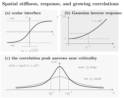
The gradient term turns a uniform order parameter into a spatial field. A scalar interface varies over a width set by $\sqrt{c/\lvert r\rvert}$; the Gaussian inverse susceptibility is $r+c k^2$; and the corresponding peak $G(k)=k_{\mathrm B}T/(r+c k^2)$ narrows as $\xi=\sqrt{c/r}$ grows.

Real-space correlator

Let

$$\kappa \equiv \xi^{-1} = \sqrt{\frac r c}.$$

In an infinite isotropic continuum,

$$G(\mathbf x) = \frac{k_{\mathrm B}T}{c} \int_{\mathbf k} \frac{e^{i\mathbf k\cdot\mathbf x}} {k^2+\kappa^2}.$$

Ignoring cutoff-sensitive contact structure at very short distance, the continuum transform is

$$\begin{aligned} G(x) ={}& \frac{k_{\mathrm B}T}{c} \frac{1}{(2\pi)^{d/2}} \\ &\times \left(\frac{\kappa}{x}\right)^{d/2-1} K_{d/2-1}(\kappa x). \end{aligned}$$

where $K_{\nu}$ is a modified Bessel function and $x=\lvert\mathbf x\rvert$. For $x\gg\xi$,

$$G(x) \propto x^{-(d-1)/2} e^{-x/\xi}.$$

In three dimensions this simplifies to

$$G(x) = \frac{k_{\mathrm B}T}{4\pi c x} e^{-x/\xi}.$$

The algebraic prefactor matters when fitting data. A pure exponential is generally not the exact continuum asymptote in more than one dimension.

Gaussian critical exponents

If $r=a_0 t$ with $t=(T-T_c)/T_c$, then

$$\xi \propto t^{-1/2},$$

so the Gaussian value is

$$\nu_{\mathrm G} = \frac12.$$

At $r=0$ and for dimensions where the Fourier transform is infrared meaningful,

$$G(k) \propto k^{-2}.$$

Comparing with the critical definition

$$G(k) \propto k^{-2+\eta}$$

gives

$$\eta_{\mathrm G} = 0.$$

These are Gaussian or mean-field values. In dimensions below the upper critical dimension, the quartic interaction generally changes them at the interacting critical fixed point.

Fluctuations in the Ordered Phase

For $r<0$, $u>0$, and $h=0$, the uniform minima are

$$\phi_0 = \pm\sqrt{\frac{\lvert r\rvert}{u}}.$$

Choose one pure phase and write

$$\phi(\mathbf x) = \phi_0 + \sigma(\mathbf x).$$

The local curvature is

$$V''(\phi_0) = r + 3u\phi_0^2 = 2\lvert r\rvert.$$

The scalar amplitude fluctuation therefore has Gaussian kernel

$$2\lvert r\rvert + c k^2$$

and longitudinal correlation length

$$\xi_- = \sqrt{\frac{c}{2\lvert r\rvert}}.$$

Above the transition at the same $\lvert r\rvert$,

$$\xi_+ = \sqrt{\frac{c}{\lvert r\rvert}},$$

so the Gaussian amplitude ratio is

$$\frac{\xi_+}{\xi_-} = \sqrt2.$$

Amplitude ratios can be universal within a universality class, but this mean-field value is not exact below the upper critical dimension.

Phase selection matters

In a finite symmetric system at zero source, averaging over both minima gives $\langle\phi\rangle=0$. Expanding about one minimum presumes a selected phase, implemented by boundary conditions, a small source followed by the thermodynamic limit, or conditioning on a sector.

Expanding around a symmetry-restored mixture is not equivalent to expanding around either pure phase. Spontaneous Symmetry Breaking owns the order of limits and phase-selection logic.

Multicomponent order and soft directions

For an $O(N)$ vector field,

$$\begin{aligned} \mathcal F[\boldsymbol\phi] = \int d^d x\, \bigg[ & \frac c2 (\nabla\boldsymbol\phi)^2 + \frac r2 \boldsymbol\phi^2 \\ &+ \frac u4 (\boldsymbol\phi^2)^2 \bigg]. \end{aligned}$$

Choose the ordered direction along component $1$ and write

$$\boldsymbol\phi = (\phi_0+\sigma,\boldsymbol\pi).$$

At quadratic order,

$$\begin{aligned} \mathcal F_2 = \frac12 \int d^d x\, \bigg[ & c(\nabla\sigma)^2 + 2\lvert r\rvert\sigma^2 \\ &+ c(\nabla\boldsymbol\pi)^2 \bigg]. \end{aligned}$$

The longitudinal amplitude mode is massive, while the $N-1$ transverse directions have no local restoring term in the symmetry-invariant approximation. Their consequences and the qualifications imposed by dimension, temperature, gauge coupling, and explicit symmetry breaking belong to Goldstone Modes in Many-Body Systems.

Interfaces and Healing

Gradient energy makes abrupt jumps costly. A domain wall illustrates how local ordering and stiffness balance.

Scalar wall equation

For $r<0$ and $h=0$, rewrite the potential relative to either minimum as

$$\begin{aligned} V(\phi)-V(\phi_0) &= \frac u4 \left(\phi^2-\phi_0^2\right)^2, \\ \phi_0^2 &= \frac{\lvert r\rvert}{u}. \end{aligned}$$

Consider a flat wall that depends only on $x$ and obeys

$$\phi(-\infty) = -\phi_0, \qquad \phi(+\infty) = \phi_0.$$

The profile equation is

$$-c\frac{d^2\phi}{dx^2} + r\phi + u\phi^3 = 0.$$

First integral

Multiplying by $d\phi/dx$ and integrating once gives

$$\frac c2 \left(\frac{d\phi}{dx}\right)^2 = V(\phi)-V(\phi_0).$$

The integration constant is fixed by the uniform limits. The equality has a mechanical analogy, but it is simply a first integral of the static Euler–Lagrange equation.

Kink profile

The exact wall is

$$\phi(x) = \phi_0 \tanh\!\left(\frac{x}{\ell_{\mathrm w}}\right),$$

with

$$\ell_{\mathrm w} = \sqrt{\frac{2c}{\lvert r\rvert}} = 2\xi_-.$$

The phrase “wall width” depends on the convention used to convert a smooth profile into one number. The intrinsic scale in the hyperbolic tangent is $\ell_{\mathrm w}$; other width definitions differ by numerical factors.

Surface tension

The excess free energy per unit wall area is

$$\begin{aligned} \sigma_{\mathrm w} = \int_{-\infty}^{\infty} dx\, \bigg[ & \frac c2 \left(\frac{d\phi}{dx}\right)^2 \\ &+ V(\phi)-V(\phi_0) \bigg]. \end{aligned}$$

Using the first integral and the kink solution yields

$$\sigma_{\mathrm w} = \frac{2\sqrt2}{3} \frac{\sqrt c\,\lvert r\rvert^{3/2}}{u}.$$

Within this mean-field theory, the wall broadens and its tension vanishes as $r\to0^-$. Close enough to a fluctuation-dominated critical point, both powers and amplitudes require corrections.

What the wall does not calculate

The static profile does not determine domain-wall mobility, damping, nucleation rate, pinning, roughening, or coarsening. Those require a dynamical law and, often, noise. Nor does the planar wall by itself provide the critical droplet for a first-order transition, whose curvature and bulk free-energy bias are essential.

The Ginzburg Criterion

Landau minimization and Gaussian fluctuations are not automatically reliable arbitrarily close to a continuous transition. The Ginzburg criterion estimates where fluctuations become comparable with the mean-field order.

Fluctuation in a correlation volume

Use the disordered-side Gaussian propagator and retain modes with $k\lesssim\xi^{-1}$. Their contribution scales as

$$\begin{aligned} \langle(\delta\phi)^2\rangle_{\xi} &\sim k_{\mathrm B}T \int_{k\lesssim\xi^{-1}} \frac{d^d k}{(2\pi)^d} \frac{1}{r+c k^2} \\ &\sim \frac{k_{\mathrm B}T}{c} \xi^{2-d}. \end{aligned}$$

Only the scaling is claimed; the numerical coefficient depends on the cutoff convention and on how the correlation volume is defined.

Below the transition, mean field gives

$$\phi_0^2 = \frac{\lvert r\rvert}{u} \sim \frac{c}{u\xi^2}.$$

The ratio is therefore

$$\frac{\langle(\delta\phi)^2\rangle_{\xi}} {\phi_0^2} \sim \frac{k_{\mathrm B}T\,u}{c^2} \xi^{4-d}.$$

Define the dimensionless fluctuation strength at scale $\xi$ by

$$g_{\xi} \equiv \frac{k_{\mathrm B}T\,u}{c^2} \xi^{4-d}.$$

Mean-field reasoning is parametrically controlled only when $g_{\xi}\ll1$.

Upper critical dimension

As $\xi\to\infty$:

• for $d<4$, $g_{\xi}$ grows and the quartic interaction becomes important;
• for $d=4$, the coupling is marginal and logarithmic corrections can appear;
• for $d>4$, $g_{\xi}$ decreases and Gaussian critical behavior is stable for the short-range scalar problem, subject to dangerous-irrelevance qualifications.

This identifies

$$d_c = 4$$

as the upper critical dimension of the ordinary short-range $\phi^4$ theory. The Renormalization Group Preview derives the same result by power counting and explains what changes at an interacting fixed point.

Width of the Ginzburg region

If

$$r = a_0 t, \qquad \xi \simeq \left(\frac{c}{a_0\lvert t\rvert}\right)^{1/2},$$

then for $d<4$,

$$g_{\xi} \sim \mathcal G \lvert t\rvert^{-(4-d)/2},$$

where

$$\mathcal G = \frac{k_{\mathrm B}T_c u}{c^2} \left(\frac{c}{a_0}\right)^{(4-d)/2}.$$

The crossover estimate $g_{\xi}\sim1$ gives

$$\lvert t_{\mathrm G}\rvert \sim \mathcal G^{2/(4-d)}.$$

This is a nonuniversal scale estimate, not a sharp phase boundary. Numerical constants, the relevant side of the transition, anisotropy, component number, interaction range, and additional soft modes all modify it.

What the criterion says and does not say

The Ginzburg criterion says when a particular mean-field expansion loses parametric control. It does not calculate the true exponents, prove that the transition remains continuous, or identify the eventual fixed point. A large Ginzburg region means non-Gaussian fluctuations matter over an experimentally visible interval; a small region can make mean-field behavior look accurate until very close to criticality.

For continuous symmetries in low dimension, transverse fluctuations introduce additional infrared constraints. For gauge-coupled or fermionic systems, integrating out other soft fields can qualitatively modify the effective functional. The scalar estimate must not be transplanted unchanged.

Multicomponent and Complex Fields

General quadratic form

For components $\phi_a$, the leading functional has the schematic form

$$\begin{aligned} \mathcal F[\boldsymbol\phi] = \int d^d x\, \bigg[ & \frac12 K_{ij}^{ab} (\partial_i\phi_a) (\partial_j\phi_b) \\ &+ V(\boldsymbol\phi) \bigg]. \end{aligned}$$

Around a stationary uniform state, the Gaussian inverse susceptibility matrix is

$$\left[\chi^{-1}(\mathbf k)\right]_{ab} = M_{ab} + K_{ij}^{ab}k_i k_j + O(k^4),$$

where

$$M_{ab} = \left. \frac{\partial^2 V} {\partial\phi_a\partial\phi_b} \right|_{\bar{\boldsymbol\phi}}.$$

Diagonalizing only $M$ may be insufficient if the stiffness matrices do not commute with it. Different eigenmodes can have different correlation lengths, polarizations, and soft wavevectors.

Complex order parameter

For a global $U(1)$ order parameter $\psi$, a neutral isotropic functional is

$$\mathcal F[\psi] = \int d^d x\, \left[ c\lvert\nabla\psi\rvert^2 + r\lvert\psi\rvert^2 + \frac u2\lvert\psi\rvert^4 \right].$$

The amplitude and phase are both spatial fields. Where $\psi\ne0$, write

$$\psi = \rho e^{i\theta}.$$

Then

$$\lvert\nabla\psi\rvert^2 = (\nabla\rho)^2 + \rho^2(\nabla\theta)^2.$$

The phase stiffness is therefore proportional to the squared amplitude in this minimal model. Singular phase configurations, compactness, and vortices require more than a smooth small-fluctuation expansion.

Gauge-covariant superconducting extension

For a charged condensate, local gauge invariance replaces the ordinary gradient by a covariant derivative and includes magnetic-field energy. Schematically,

$$\begin{aligned} \mathcal F[\psi,\mathbf A] ={}& \int d^3 x\, \bigg\{ c\left\lvert \left(\nabla-iq\mathbf A\right)\psi \right\rvert^2 \\ &+ r\lvert\psi\rvert^2 + \frac u2\lvert\psi\rvert^4 + \frac{\mathbf B^2}{2\mu_0} \bigg\}. \end{aligned}$$

Factors of $\hbar$ and charge depend on how $c$, $q$, and $\psi$ are defined. The gauge field is dynamical within the equilibrium functional and can change both collective modes and fluctuation physics. Ginzburg–Landau Theory owns the superconducting material application, including its normalization ledger, coherence and penetration lengths, critical fields, type criterion, and vortices.

Coupled orders

Several order parameters can share gradients and local couplings. For two scalars,

$$\begin{aligned} \mathcal F = \int d^d x\, \bigg[ & \frac{c_\phi}{2}(\nabla\phi)^2 + \frac{c_\psi}{2}(\nabla\psi)^2 \\ &+ V(\phi,\psi) \bigg]. \end{aligned}$$

A local term $w\phi^2\psi^2$ can favor competition or coexistence, while derivative couplings can mix spatial modes. The uniform phase topology remains the responsibility of Landau theory; the present extension determines how the coupled orders vary and fluctuate in space.

Thermal, Quantum, and Dynamical Theories

Static thermal field theory

The integral

$$\mathcal Z = \int\mathcal D\phi\, e^{-\beta\mathcal F[\phi]}$$

is a $d$-dimensional classical statistical field theory. It can describe the long-distance static sector of a finite-temperature quantum many-body system when nonzero Matsubara modes and other massive fields have been integrated out appropriately.

The resulting coefficients contain quantum and thermal short-distance physics. Calling the final field theory “classical” refers to the statistical form of the remaining static modes, not to the microscopic constituents.

Quantum critical action

A zero-temperature quantum transition generally needs an imaginary-time-dependent field:

$$\mathcal Z = \int\mathcal D\phi\, e^{-S_{\mathrm E}[\phi]/\hbar}.$$

A schematic local action might contain

$$\begin{aligned} S_{\mathrm E} = \int d\tau\,d^d x\, \bigg[ & \frac{Z_\tau}{2} (\partial_\tau\phi)^2 \\ &+ \frac c2(\nabla\phi)^2 + V(\phi) \bigg]. \end{aligned}$$

but many-body systems can instead produce first-order time derivatives, Landau damping, Berry phases, nonlocal kernels, or gauge constraints. The dynamical exponent $z$ and the effective dimension $d+z$ cannot be inferred from the static functional alone.

Quantum Phase Transitions owns the scaling distinction between thermal and quantum criticality. Why Many-Body QM Leads to QFT develops the broader route from microscopic, auxiliary, and collective fields to effective actions.

Static functional does not imply kinetics

Two systems can share the same equilibrium $\mathcal F[\phi]$ but have different dynamics because the order parameter may be conserved in one system and nonconserved in another, or because it couples to momentum, energy, gauge fields, or other slow variables.

An equation such as

$$\partial_t\phi = -\Gamma \frac{\delta\mathcal F}{\delta\phi}$$

is an additional relaxational model, not a consequence of the equilibrium functional. Noise and fluctuation–dissipation consistency must also be specified. Dynamic universality is a separate classification problem.

From Microscopic Physics to the Functional

Symmetry constrains; matching determines

Symmetry tells which local and derivative operators may appear. It does not determine their coefficients. Microscopic matching may use:

• a controlled expansion near weak coupling;
• a Hubbard–Stratonovich transformation followed by integrating out matter fields;
• a cumulant or linked-cluster expansion;
• density-functional or effective-action methods;
• measured susceptibilities, stiffnesses, and nonlinear response;
• numerical coarse-graining.

The same symmetry class can therefore have very different $c$, $u$, cutoff, Ginzburg window, and nonuniversal amplitudes.

Auxiliary and collective fields are not synonyms

An auxiliary field can be introduced through an exact integral identity. It becomes a collective order-parameter field only after one identifies its transformation properties, source coupling, saddle, fluctuations, and relation to observables. Integrating out microscopic matter can also generate a nonlocal or complex effective action rather than the simple local real functional assumed here.

Derivative and amplitude expansions are independent

Small gradients do not guarantee small amplitude, and small amplitude does not guarantee slow variation. A controlled local theory needs both relevant expansions to be valid in the regime used:

$$\frac{\lvert\nabla\phi\rvert}{\Lambda\lvert\phi\rvert} \ll 1$$

where meaningful, together with suppression of omitted powers of $\phi$. Near a defect core, boundary, or first-order interface, one expansion can fail before the other.

Coefficients depend on scale

Integrating out fluctuations between two cutoffs changes the effective coefficients and generates every operator allowed by symmetry. A polynomial that is accurate at one coarse-graining scale need not retain the same numerical coefficients at another.

This is why the Landau–Ginzburg functional is the starting point, not the endpoint, of the Wilsonian analysis. The one-canonical-home continuation is Renormalization Group Preview.

Representative Uses

Ising-like magnets and binary mixtures

A real scalar field can represent coarse-grained magnetization or a composition difference. The source is a magnetic field or chemical-potential difference, the stiffness penalizes spatial variation, and the Gaussian peak describes long-wavelength critical scattering above the transition.

The mapping identifies symmetry and soft modes, not numerical equality of coefficients. A fluid near its liquid–gas critical endpoint has no microscopic spin-inversion symmetry, but field mixing can produce an emergent scalar critical description.

Structural transitions

A displacement, strain component, or orientational tensor can serve as the order parameter. Crystal symmetry controls invariant polynomials and anisotropic gradients. Compatibility constraints and elastic long-range interactions can make the effective kernel nonlocal, so a naive local $c k^2$ approximation may be insufficient.

Neutral condensates

A complex field describes amplitude and phase variations of a neutral condensate. The stationary Gross–Pitaevskii equation has a related gradient-plus-local-nonlinearity structure, but its coefficients and interpretation arise from a condensate wavefunction and particle-number constraint. Gross–Pitaevskii Equation owns that microscopic mean-field setting, healing length, and condensate dynamics.

Superconductors

The charged complex functional predicts coherence and magnetic screening scales, interfaces, vortices, and critical fields once electromagnetic coupling and material parameters are included. Near an ordinary thermal transition it can often be matched to microscopic BCS theory, but the phenomenological construction itself does not assume BCS pairing.

Modulated phases

Competing interactions may soften modes near $\mathbf Q\ne0$. Then the correct field may be a complex amplitude multiplying $e^{i\mathbf Q\cdot\mathbf x}$, a collection of symmetry-related wavevectors, or a tensor. Keeping the wavevector structure prevents the gradient expansion from misclassifying translation-breaking order.

What the Theory Predicts Reliably

Within a controlled regime, a Landau–Ginzburg functional can organize:

• allowed local and gradient terms;
• stationary textures and boundary profiles;
• the relation between stiffness, curvature, and Gaussian correlation lengths;
• momentum-dependent static response;
• mean-field interfaces and surface tension;
• which modes become soft;
• a starting action for fluctuation and RG calculations;
• dimensional estimates of where mean field fails.

Its most robust output is often structural: which fields and operators must be retained, what symmetry relates them, and what scales can be formed from the coefficients.

Limitations and Breakdown

Fluctuation-dominated criticality

Below $d_c=4$ for short-range scalar $\phi^4$ theory, Gaussian exponents are generally not the asymptotic ones. The Ginzburg criterion locates a crossover estimate but does not replace RG or high-precision numerical and experimental analysis.

Low-dimensional continuous symmetry

Massless angular fluctuations can prevent conventional finite-temperature long-range order under the hypotheses of the Mermin–Wagner–Hohenberg results. A saddle with $\lvert\boldsymbol\phi\rvert\ne0$ does not by itself prove that the thermal expectation value remains ordered.

Topological defects

Smooth Gaussian expansion around one field value misses changes of winding sector, vortex cores, domain-wall proliferation, and other defect physics. Defects can control transitions even when a local field remains useful.

Additional soft degrees of freedom

Coupling an order parameter to gauge fields, conserved densities, phonons, or gapless fermions can generate nonanalytic kernels, alter exponents, or drive a transition first order. Integrating these modes out is legitimate only when their effects remain local and controlled at the scales of interest.

Strong first-order transitions

An amplitude expansion around zero may not cover distant competing minima. Interfaces can sample field values outside the polynomial’s reliable range. A phenomenological fit to equilibrium minima does not automatically predict the barrier or nucleation path.

Disorder and inhomogeneity

Random mass, random field, dilution, strain, and boundaries introduce spatially varying coefficients and new fluctuation regimes. Replacing disorder by its average can erase rare regions or change the symmetry of the effective problem.

Ultraviolet dependence

Coincident correlators and fluctuation determinants are cutoff dependent. A continuum integral extended to infinite momentum can diverge even though the original lattice model is finite. Regulate first, match coefficients consistently, and distinguish universal infrared behavior from ultraviolet-sensitive amplitudes.

Nonequilibrium and open systems

An equilibrium free-energy functional need not exist for a driven steady state. Even when a Lyapunov functional exists, it may not generate the probability distribution or response relations assumed above. Real-time contours, noise statistics, and conservation laws must be supplied explicitly.

Phases beyond local symmetry breaking

Topological order and intrinsically nonlocal organization cannot be classified completely by minimizing a local order-parameter field. The next Topological Order Preview marks this boundary without replacing the dedicated Quantum Matter treatment.

A Reliable Workflow

1. Define the observable field

State the microscopic operator or constrained variable, its normalization, components, transformation law, and conjugate source.

2. Identify the soft wavevectors

Determine whether the instability occurs at $\mathbf k=0$, at isolated nonzero $\mathbf Q$, on a shell, or along a larger low-energy manifold.

3. Declare the coarse-graining scale

Specify the cutoff or cell size and the separation between microscopic and collective scales. Do not use the continuum functional below its resolution.

4. Enumerate allowed operators

Apply internal, spatial, time-reversal, lattice, and gauge symmetries to both local powers and derivatives. Include every term of the retained order that symmetry permits.

5. Check boundedness and the full quadratic spectrum

Verify stability at large amplitude and for every allowed momentum and component. A positive local quartic does not repair a gradient sector that runs to negative infinity.

6. Separate saddle predictions from fluctuation predictions

Label uniform minimization, inhomogeneous stationarity, Gaussian integration, loop corrections, and RG results distinctly.

7. Match response conventions

Track factors of $\beta$, volume, Fourier normalization, and field units. State whether a plotted quantity is $G(k)$, $\chi(k)$, or an experimental structure factor.

8. Test infrared control

Estimate the Ginzburg parameter, inspect Goldstone or gauge modes, and compare the correlation length with system size and other infrared cutoffs.

9. Test ultraviolet control

Check that dominant momenta lie below $\Lambda$, omitted derivatives remain small, and loop integrals use the same regulator as coefficient matching.

10. Compare with independent observables

Use susceptibility, correlation length, scattering line shape, stiffness, interface width, finite-size scaling, or microscopic numerics as cross-checks rather than fitting one curve in isolation.

Common Mistakes

Calling a saddle-point profile an exact thermal average

The Euler–Lagrange solution is the most probable or stationary coarse-grained profile under stated conditions. Fluctuations can shift, broaden, or qualitatively invalidate it.

Omitting the cutoff

A local continuum functional is an effective theory. Sending every loop or variance integral to infinite momentum while keeping phenomenological coefficients fixed is inconsistent.

Confusing correlations with susceptibility

In the present classical equilibrium convention, $G(k)=k_{\mathrm B}T\chi(k)$. Other normalizations may include volume or density factors.

Treating every correlation length as the Gaussian pole length

That expression is the Gaussian pole length of a particular mode. Interacting, anisotropic, multicomponent, finite-size, and second-moment lengths require their own definitions and may differ away from scaling.

Ignoring boundary variations

Integration by parts produces a surface term. A bulk equation without a compatible boundary condition does not define the variational problem.

Assuming positive stiffness by habit

The sign and tensor structure of the stiffness follow from the microscopic kernel. A negative eigenvalue can signal finite-wavevector order and demands higher gradients or a different expansion point.

Reading dynamics from a static functional

The free-energy landscape does not determine whether the order parameter propagates, diffuses, precesses, or relaxes, nor whether it is conserved.

Using mean-field exponents inside the Ginzburg region

The criterion is specifically a warning that the Gaussian approximation is losing control. Quoting $\nu=1/2$ there as an exact prediction reverses its meaning.

Treating the Ginzburg scale as a new transition

$t_{\mathrm G}$ is a crossover estimate. It is convention dependent and has no independent thermodynamic singularity.

Equating a complex field with superconductivity

A neutral superfluid also has a complex order parameter. Superconductivity additionally requires charge, gauge coupling, electromagnetic energy, and the appropriate material matching.

Forgetting other soft fields

Integrating out a gapless mode can generate nonlocality. A tidy local polynomial is not evidence that the omitted field was harmless.

Exercises

Exercise 1: Physical units

For

$$\begin{aligned} \mathcal F = \int d^d x\, \bigg[ & \frac c2(\nabla\phi)^2 + \frac r2\phi^2 \\ &+ \frac u4\phi^4 - h\phi \bigg]. \end{aligned}$$

derive the physical units of $c$, $r$, $u$, and $h$ in terms of energy, length, and the unit of $\phi$. Show directly that

$$\frac{k_{\mathrm B}T\,u}{c^2} \xi^{4-d}$$

is dimensionless.

Solution

The gradient term gives

$$[c] [\phi]^2 [L]^{d-2} = [E],$$

so

$$[c] = [E][L]^{2-d}[\phi]^{-2}.$$

The remaining terms give

$$\begin{aligned} [r] &= [E][L]^{-d}[\phi]^{-2}, \\ [u] &= [E][L]^{-d}[\phi]^{-4}, \\ [h] &= [E][L]^{-d}[\phi]^{-1}. \end{aligned}$$

Therefore

$$\left[ \frac{k_{\mathrm B}T\,u}{c^2} \right] = [L]^{d-4},$$

and multiplication by $\xi^{4-d}$ removes the remaining length unit. This check would fail if $\mathcal F$ and $\beta\mathcal F$ conventions were mixed.

Exercise 2: Sinusoidal source

In the disordered Gaussian theory, apply

$$h(\mathbf x) = h_0\cos(\mathbf q\cdot\mathbf x).$$

Find the stationary linear-response profile. Explain the limits $q\xi\ll1$ and $q\xi\gg1$.

Solution

The linear equation is

$$\left(-c\nabla^2+r\right)\phi = h_0\cos(\mathbf q\cdot\mathbf x).$$

Because the source is a Laplacian eigenfunction, take

$$\phi(\mathbf x) = \phi_q\cos(\mathbf q\cdot\mathbf x).$$

Substitution gives

$$\phi_q = \frac{h_0}{r+c q^2} = \frac{h_0/r}{1+q^2\xi^2}.$$

For $q\xi\ll1$, the source varies slowly across a correlation length and the response approaches the uniform value $h_0/r$. For $q\xi\gg1$, stiffness suppresses the response as $h_0/(c q^2)$. The crossover directly measures the pole length $\xi$ in the Gaussian approximation.

Exercise 3: Three-dimensional Gaussian correlator

Starting from

$$G(\mathbf k) = \frac{k_{\mathrm B}T}{r+c k^2},$$

show that for $x>0$ in three dimensions,

$$G(x) = \frac{k_{\mathrm B}T}{4\pi c x} e^{-x/\xi}.$$

Why is the expression not trustworthy at arbitrarily small $x$?

Solution

Choose the polar axis along $\mathbf x$. The angular integral gives

$$G(x) = \frac{k_{\mathrm B}T}{2\pi^2 c x} \int_0^{\infty} dk\, \frac{k\sin(kx)}{k^2+\xi^{-2}}.$$

For $x>0$,

$$\int_0^{\infty} dk\, \frac{k\sin(kx)}{k^2+\xi^{-2}} = \frac{\pi}{2}e^{-x/\xi}.$$

Combining factors yields

$$G(x) = \frac{k_{\mathrm B}T}{4\pi c x} e^{-x/\xi}.$$

The derivation extended the small-$k$ kernel to infinite momentum. At distances comparable with the coarse-graining cell, the cutoff and higher-gradient terms change the result. The $1/x$ divergence is therefore not a literal prediction at $x=0$.

Exercise 4: Domain wall

For $r<0$, verify the profile

$$\phi(x) = \sqrt{\frac{\lvert r\rvert}{u}} \tanh\!\left( x\sqrt{\frac{\lvert r\rvert}{2c}} \right).$$

Then derive its surface tension.

Solution

Let

$$\phi_0 = \sqrt{\frac{\lvert r\rvert}{u}}, \qquad \ell_{\mathrm w} = \sqrt{\frac{2c}{\lvert r\rvert}}.$$

For $\phi=\phi_0\tanh(x/\ell_{\mathrm w})$, direct differentiation gives

$$-c\phi'' - \lvert r\rvert\phi + u\phi^3 = 0.$$

The first integral implies

$$\frac c2(\phi')^2 = V(\phi)-V(\phi_0),$$

so the two contributions to the wall energy are equal and

$$\sigma_{\mathrm w} = c \int_{-\infty}^{\infty} dx\, (\phi')^2.$$

Using

$$\phi' = \frac{\phi_0}{\ell_{\mathrm w}} \operatorname{sech}^2 \!\left(\frac{x}{\ell_{\mathrm w}}\right)$$

and

$$\int_{-\infty}^{\infty}dy\, \operatorname{sech}^4 y = \frac43$$

gives

$$\sigma_{\mathrm w} = \frac{2\sqrt2}{3} \frac{\sqrt c\,\lvert r\rvert^{3/2}}{u}.$$

Exercise 5: Ginzburg criterion and dimension

Use

$$\langle(\delta\phi)^2\rangle_{\xi} \sim \frac{k_{\mathrm B}T}{c}\xi^{2-d}$$

and

$$\phi_0^2 \sim \frac{c}{u\xi^2}$$

to classify the fluctuation correction for $d=3$, $d=4$, and $d=5$. Why does the estimate alone not prove mean-field theory exact in five dimensions for every observable?

Solution

The ratio scales as

$$g_{\xi} \sim \frac{k_{\mathrm B}T u}{c^2} \xi^{4-d}.$$

Thus:

$$\begin{array}{c|c|c} d & g_{\xi}\text{ as }\xi\to\infty & \text{interpretation} \\ \hline 3 & \propto\xi & \text{grows} \\ 4 & \propto\xi^0 & \text{marginal estimate} \\ 5 & \propto\xi^{-1} & \text{decreases} \end{array}$$

In three dimensions the Gaussian approximation eventually fails. In four dimensions the scaling estimate is inconclusive about logarithms, so nonlinear RG is required. In five dimensions Gaussian exponents are stable for the short-range scalar critical point, but the quartic coupling can be dangerously irrelevant for order-parameter and finite-size scaling. The Ginzburg estimate also assumes that no other soft fields or nonlocal interactions intervene.

Exercise 6: Anisotropic correlation lengths

Let

$$\mathcal F_2 = \frac12 \int d^d x\, \left[ r\phi^2 + \sum_{i=1}^{d} c_i(\partial_i\phi)^2 \right],$$

with every $c_i>0$. Find the Gaussian susceptibility and the principal correlation lengths. Show how a coordinate rescaling makes the quadratic kernel isotropic.

Solution

Fourier transformation gives

$$\chi(\mathbf k) = \frac{1} {r+\sum_i c_i k_i^2}.$$

Along principal axis $i$, the pole length is

$$\xi_i = \sqrt{\frac{c_i}{r}}.$$

Choose a reference stiffness $c_*$ and define

$$x_i' = x_i\sqrt{\frac{c_*}{c_i}}.$$

Then derivatives transform so that the gradient kernel becomes proportional to

$$c_* \sum_i (\partial_i'\phi)^2,$$

while the Jacobian changes the overall coefficient normalization. This removes quadratic anisotropy in the bulk continuum theory, but lattice anisotropies can survive in higher derivatives, boundaries, observables, or as relevant perturbations at other fixed points.

Exercise 7: Finite-wavevector instability

Consider

$$K(k) = r + c k^2 + \kappa k^4, \qquad \kappa>0.$$

Find the soft wavevector for $c>0$, $c=0$, and $c<0$. For $c<0$, determine the value of $r$ at which the minimum of $K(k)$ first reaches zero.

Solution

Stationary wave numbers satisfy

$$\frac{dK}{dk} = 2k \left(c+2\kappa k^2\right) = 0.$$

For $c>0$, the minimum is at $k=0$. At $c=0$, the leading dispersion is quartic and $k=0$ remains the minimum. For $c<0$, the nonzero minimum is

$$q_0^2 = -\frac{c}{2\kappa}.$$

At this wave number,

$$K(q_0) = r - \frac{c^2}{4\kappa}.$$

The Gaussian instability therefore occurs at

$$r = \frac{c^2}{4\kappa}.$$

The result shows why setting the quartic-gradient term to zero when $c<0$ makes the continuum theory unbounded and loses the modulation scale.

Exercise 8: Classify four field theories

Classify each expression as a static thermal functional, a Euclidean quantum action, or an added dynamical law. State one piece of information missing from each schematic formula.

$$\text{(a)}\qquad \mathcal Z = \int\mathcal D\phi\, e^{-\beta\mathcal F[\phi]}.$$ $$\begin{aligned} \text{(b)}\qquad & \\ S_{\mathrm E} &= \int d\tau\,d^d x\, \big[ & (\partial_\tau\phi)^2 \\ &+ (\nabla\phi)^2 + V(\phi) \big]. \end{aligned}$$ $$\text{(c)}\qquad \partial_t\phi = -\Gamma \frac{\delta\mathcal F}{\delta\phi}.$$ $$\begin{aligned} \text{(d)}\qquad \mathcal F = \int d^3 x\, \big[ & \lvert(\nabla-iq\mathbf A)\psi\rvert^2 \\ &+ V(\lvert\psi\rvert) + \frac{\mathbf B^2}{2\mu_0} \big]. \end{aligned}$$

Solution

• (a) is a static thermal field integral. It still needs a cutoff, measure, coefficient convention, and boundary conditions.
• (b) is a schematic Euclidean quantum action. It still needs the coefficient normalization, temporal boundary conditions, regulator, and justification for the quadratic time derivative.
• (c) is an added deterministic relaxational law. It still needs the conservation class, noise, mobility structure, and fluctuation–dissipation relation if equilibrium is intended.
• (d) is a static gauge-coupled Ginzburg–Landau functional. It still needs charge and $\hbar$ conventions, electromagnetic boundary conditions, material coefficients, and a statement of whether gauge-field fluctuations are integrated over or treated classically.

The exercise emphasizes that similar-looking gradient terms do not determine the physical interpretation by themselves.

Key Takeaways

• Landau–Ginzburg theory replaces a uniform order parameter by a coarse-grained spatial field with a declared ultraviolet cutoff.
• The gradient term is the leading small-momentum dependence of the inverse susceptibility when locality, analyticity, and a $k=0$ soft mode apply.
• The Gaussian kernel $r+c k^2$ gives $\chi(k)=1/(r+c k^2)$ and $\xi=\sqrt{c/r}$ above the transition.
• Gaussian criticality predicts $\nu=1/2$ and $\eta=0$, but these values generally fail below four dimensions sufficiently near an interacting critical point.
• Minimizing the functional is a saddle-point approximation; integrating over configurations adds fluctuations.
• The scalar theory predicts a smooth domain wall whose width scales as $\sqrt{c/\lvert r\rvert}$ and whose tension scales as $\sqrt c\lvert r\rvert^{3/2}/u$.
• The Ginzburg parameter $g_{\xi}\sim(k_{\mathrm B}T u/c^2)\xi^{4-d}$ estimates where mean field loses control and identifies $d_c=4$ for short-range $\phi^4$ theory.
• Boundaries, anisotropy, finite-wavevector order, gauge fields, Goldstone modes, disorder, and other soft degrees of freedom can require a larger or nonlocal theory.
• A static equilibrium functional does not specify dynamics or quantum imaginary-time structure.

Further Reading

• Landau Theory for the canonical uniform invariant expansion and mean-field thermodynamics.
• Connected Correlation Functions for exponential, effective, and second-moment correlation lengths.
• Structure Factors for momentum-space observables and scattering conventions.
• Critical Exponents and Scaling for exponent definitions and non-Gaussian scaling forms.
• Renormalization Group Preview for coupling flows, upper critical dimensions, and fixed points.
• Path Integrals for Statistical Mechanics for deriving thermal functional integrals from quantum traces.
• Why Many-Body QM Leads to QFT for microscopic, auxiliary, and collective fields.
• Quantum Phase Transitions for imaginary time, dynamical scaling, and quantum-critical regimes.
• Vortex Matter, Pinning, and Flux Flow for the material-scale collective, disordered, thermally activated, and driven physics that begins after a static superconducting vortex solution is available.

References

1. V. L. Ginzburg and L. D. Landau, “On the Theory of Superconductivity,” Zhurnal Eksperimental’noi i Teoreticheskoi Fiziki 20, 1064–1082 (1950); English reprint in Collected Papers of L. D. Landau, doi:10.1016/B978-0-08-010586-4.50078-X.
2. M. E. Fisher, “Correlation Functions and the Critical Region of Simple Fluids,” Journal of Mathematical Physics 5, 944–962 (1964), doi:10.1063/1.1704197.
3. M. E. Fisher, “The Theory of Equilibrium Critical Phenomena,” Reports on Progress in Physics 30, 615–730 (1967), doi:10.1088/0034-4885/30/2/306.
4. K. G. Wilson, “Renormalization Group and Critical Phenomena. I. Renormalization Group and the Kadanoff Scaling Picture,” Physical Review B 4, 3174–3183 (1971), doi:10.1103/PhysRevB.4.3174.
5. K. G. Wilson, “Renormalization Group and Critical Phenomena. II. Phase-Space Cell Analysis of Critical Behavior,” Physical Review B 4, 3184–3205 (1971), doi:10.1103/PhysRevB.4.3184.
6. D. J. Amit, D. J. Bergman, and Y. Imry, “The Wilson Theory and the Ginzburg Critical Region,” Journal of Physics C: Solid State Physics 6, 2685–2690 (1973), doi:10.1088/0022-3719/6/17/010.
7. K. G. Wilson and J. Kogut, “The Renormalization Group and the $\epsilon$ Expansion,” Physics Reports 12, 75–199 (1974), doi:10.1016/0370-1573(74)90023-4.
8. K. G. Wilson, “The Renormalization Group: Critical Phenomena and the Kondo Problem,” Reviews of Modern Physics 47, 773–840 (1975), doi:10.1103/RevModPhys.47.773.
9. P. C. Hohenberg and B. I. Halperin, “Theory of Dynamic Critical Phenomena,” Reviews of Modern Physics 49, 435–479 (1977), doi:10.1103/RevModPhys.49.435.
10. P. M. Chaikin and T. C. Lubensky, Principles of Condensed Matter Physics, Cambridge University Press (1995), doi:10.1017/CBO9780511813467.
11. J. Cardy, Scaling and Renormalization in Statistical Physics, Cambridge University Press (1996), doi:10.1017/CBO9781316036440.
12. N. Goldenfeld, Lectures on Phase Transitions and the Renormalization Group, CRC Press reissue, doi:10.1201/9780429493492.
13. M. Kardar, Statistical Physics of Fields, Cambridge University Press (2007), doi:10.1017/CBO9780511815881.
14. J. P. Sethna, Statistical Mechanics: Entropy, Order Parameters, and Complexity, 2nd ed., Oxford University Press (2021), doi:10.1093/oso/9780198865247.001.0001.
15. B. Rosenstein and D. Li, Ginzburg–Landau Theory of Condensates, Cambridge University Press (2021), doi:10.1017/9781108872737.
16. B. I. Halperin, T. C. Lubensky, and S.-K. Ma, “First-Order Phase Transitions in Superconductors and Smectic-A Liquid Crystals,” Physical Review Letters 32, 292–295 (1974), doi:10.1103/PhysRevLett.32.292.