Universality

Universality is the principle that distinct microscopic systems can share the same asymptotic long-distance behavior near a continuous transition. A universality class is the corresponding equivalence class of critical points, not an equivalence class of complete Hamiltonians or phase diagrams.

For two systems $A$ and $B$, the microscopic lattice, coupling constants, critical temperature, and raw amplitudes may differ. Nevertheless, sufficiently close to their critical points they can have:

• the same critical exponents;
• the same properly normalized scaling functions;
• the same selected amplitude ratios;
• the same long-distance symmetry and operator content;
• the same pattern of relevant perturbations.

The qualification properly normalized matters. If

$$\xi_i(t_i) \sim \xi_{0,i}^{\pm} \lvert t_i\rvert^{-\nu}, \qquad i\in\{A,B\},$$

then the exponent $\nu$ may be common while the correlation-length amplitudes $\xi_{0,A}^{\pm}$ and $\xi_{0,B}^{\pm}$ are not. Universality begins after microscopic units and other nonuniversal metric factors have been separated from the singular structure.

This principle is powerful because a solvable model, continuum field theory, simulation, or experiment can then teach us about many systems at once. It is also easy to overstate. Symmetry and dimensionality are central classifiers, but they do not by themselves guarantee a class: interaction range, order-parameter representation, allowed perturbations, disorder, conservation laws, topological defects, and additional gapless modes can all matter.

Canonical Scope

This page is the canonical home for:

• the definition of a universality class;
• the distinction between universal and nonuniversal data;
• the role of symmetry, spatial dimension, interaction range, and order-parameter structure;
• static, dynamic, bulk, boundary, thermal, and quantum universality;
• standard examples and counterexamples;
• a defensible workflow for proposing and testing a universality class.

Neighboring pages retain separate ownership:

• Critical Exponents and Scaling owns the exponent dictionary, homogeneous scaling, finite-size scaling, correction terms, and data-collapse methodology; the Critical Exponent Glossary provides a compact assumption-aware lookup.
• Finite-Temperature Phase Transitions owns thermal transition order, coexistence, and thermodynamic singularities.
• Quantum Phase Transitions owns zero-temperature criticality, quantum-critical fans, and benchmark Hamiltonians.
• Order Parameters owns operator, source, component, and normalization choices.
• Emergent Symmetry owns enlargement of symmetry at long distances.
• Mean-Field Theory owns self-consistent approximations and their fluctuation limits.
• Renormalization Group Preview owns coarse-graining maps, fixed points, flow diagrams, and relevant, irrelevant, and marginal directions in depth. This page uses that language only to explain classification.
• Critical Phenomena and RG Bridge owns the continuum scaling limit and the matching of microscopic observables to fixed-point operators.

What a Universality Class Is

A statement about a limit

Universality is asymptotic. Let $u$ denote a relevant control that vanishes at a continuous critical point, and let $\xi(u)$ be the largest equilibrium correlation length. The universal regime requires

$$a \ll \ell \ll \xi(u),$$

where $a$ is a microscopic length and $\ell$ is an observation or coarse-graining scale. At fixed $u\ne0$, the window disappears once $\ell$ approaches $\xi$. At the critical point, $\xi$ diverges and a scale-invariant regime can persist to arbitrarily large $\ell$ in the thermodynamic limit.

Two microscopic systems belong to the same universality class only with respect to specified critical points and specified long-distance observables. This is a local statement in parameter space. One Hamiltonian can contain several transitions belonging to different classes.

An equivalence after metric factors

A useful schematic scaling form for an observable $O$ is

$$\begin{aligned} O_i^{\mathrm{sing}} (u_i,h_i,L_i) &= A_{O,i}b^{-x_O} \\ &\quad\times \mathcal F_O \left( c_{u,i}u_i b^{y_u}, \right. \\ &\qquad\left. c_{h,i}h_i b^{y_h}, \right. \\ &\qquad\left. \frac{L_i}{b}, \ldots \right). \end{aligned}$$

Here:

• $i$ labels the microscopic system;
• $A_{O,i}$, $c_{u,i}$, and $c_{h,i}$ are nonuniversal metric factors;
• $x_O$, $y_u$, and $y_h$ are universal scaling dimensions or eigenvalues for the class;
• $\mathcal F_O$ is universal only after normalization, geometry, and boundary conditions are fixed;
• the omitted arguments include irrelevant fields and other controls.

The microscopic systems need not share the same bare couplings. The class is identified by the common asymptotic data that remain after the system-dependent factors are removed.

Not an identity of whole models

The statement

“The transverse-field Ising chain and the two-dimensional classical Ising model share a critical universality class”

does not mean that their spectra, finite-temperature phase diagrams, real-time dynamics, microscopic operators, or all correlation functions are identical. It means that a specified zero-temperature critical point of the chain and the thermal critical point of the classical model share an appropriate long-distance critical theory after the quantum-to-classical correspondence and operator dictionary are established.

Universality therefore does not erase microscopic physics. It organizes which microscopic details control leading singular behavior and which instead survive in crossover scales, amplitudes, analytic backgrounds, or corrections.

Universal and Nonuniversal Data

Commonly universal

Within a fixed class and with the needed conventions stated, universal data can include:

• critical exponents such as $\nu$, $\eta$, and $\beta_{\mathrm{op}}$;
• scaling dimensions and the spectrum of long-distance operators;
• properly normalized scaling functions;
• selected ratios of critical amplitudes;
• fixed-point values of dimensionless quantities for fixed geometry and boundary conditions;
• the topology of the order-parameter manifold and its stable defect types;
• central charges and operator-product data when a conformal description applies.

Even this list needs conditions. A Binder ratio at criticality, for example, depends on shape, boundary condition, and the definition of the order parameter. It is universal only within that specified setup.

Commonly nonuniversal

The following usually retain microscopic information:

• the numerical critical temperature $T_c$ or coupling $g_c$;
• lattice spacing, bandwidth, velocity, and ultraviolet cutoff;
• raw order-parameter, susceptibility, and correlation-length amplitudes;
• analytic background terms;
• the width of the experimentally accessible scaling window;
• coefficients of irrelevant corrections;
• crossover locations away from the asymptotic critical region.

An individual amplitude can become useful in a universal ratio. If

$$\xi(t) \sim \begin{cases} \xi_0^+ t^{-\nu}, & t\to0^+,\\ \xi_0^- (-t)^{-\nu}, & t\to0^-, \end{cases}$$

then $\xi_0^+$ and $\xi_0^-$ depend on microscopic length units, but

$$R_\xi := \frac{\xi_0^+}{\xi_0^-}$$

can be universal after the definitions of $\xi$ and $t$ are fixed.

A practical dictionary

Question	Usually universal?	Required qualification
Is the critical exponent $\nu$ shared?	Yes	Same class and asymptotic regime
Is $T_c$ shared?	No	It depends on microscopic energy scales
Is a raw susceptibility amplitude shared?	No	Field and operator normalizations differ
Is an amplitude ratio shared?	Often	Definitions and scaling fields must match
Is a normalized scaling curve shared?	Often	Metric factors, shape, and boundaries must match
Is the dynamic exponent $z$ shared?	Not from statics alone	Dynamic rules and conserved quantities must match
Is a finite-size crossing value shared?	Conditionally	Same observable, aspect ratio, and boundary class

Why Microscopic Details Can Disappear

Imagine replacing blocks of nearby microscopic variables by collective variables. Repeating this operation changes the effective couplings used to describe longer scales. The correlation length in microscopic units shrinks under each rescaling, while the description retains only those combinations of couplings that continue to influence long-distance observables.

Near a continuous critical point, three broad kinds of perturbation occur:

1. Relevant perturbations grow under coarse-graining and must be tuned or specified.
2. Irrelevant perturbations shrink and affect corrections rather than the leading asymptotic behavior.
3. Marginal perturbations require further analysis because they may drift logarithmically, remain continuously variable, or become marginally relevant or irrelevant.

Microscopic models can begin at different coupling values yet approach the same long-distance fixed structure once the relevant controls are tuned. Their irrelevant couplings remember the lattice or short-distance interaction, but that memory decays with scale.

This is the mechanism behind universality, not a claim that every microscopic coupling is unimportant. A perturbation that is irrelevant at one fixed point may be relevant at another. A weak anisotropy, long-range tail, random field, or coupling to gapless fermions must be classified rather than dismissed by size alone.

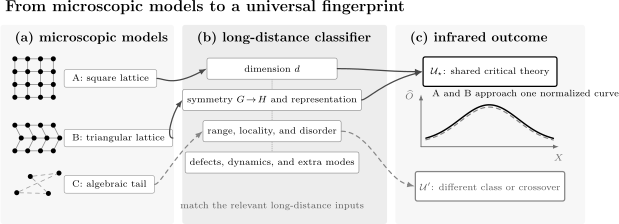
Universality is a many-to-one long-distance statement. Distinct microscopic models can share a critical fingerprint after the critical point is tuned and the relevant classification data are matched. Changing dimension, symmetry representation, interaction range, disorder, or dynamics can redirect the flow to a different class or away from a continuous transition.

Classification Is a Structured Question

A useful first-pass label is not merely “Ising-like” or “continuous.” It records enough information to identify the proposed infrared problem:

$$\begin{gathered} \mathcal U \sim \left( d,\, G\to H,\, \mathcal R_\phi,\, \right. \\ \left. \text{range},\, \text{locality},\, \text{defects},\, \right. \\ \left. \text{disorder},\, \text{dynamics},\, \text{extra modes} \right). \end{gathered}$$

Here $d$ is spatial dimension, $G\to H$ is the symmetry-breaking pattern when one exists, and $\mathcal R_\phi$ is the representation and component structure of the order parameter. This tuple is a checklist, not a theorem or a complete invariant. Some critical points have no local order parameter, and distinct fixed points can share the same obvious entries.

Spatial Dimensionality

Dimension changes both the phase structure and the strength of fluctuations.

Lower critical dimensions

Below a lower critical dimension $d_\ell$, fluctuations prevent the ordered phase or transition assumed by a naive local order-parameter theory. Examples include:

• the one-dimensional short-range classical Ising model, which has no finite-temperature ordering transition;
• short-range systems with a continuous symmetry, for which thermal fluctuations forbid conventional long-range order in $d\le2$ under the hypotheses of the Mermin–Wagner theorem.

The second example does not mean “nothing happens” in two dimensions. The two-dimensional XY model supports a Berezinskii–Kosterlitz–Thouless transition controlled by vortex unbinding and an essential correlation-length singularity. That is precisely why dimension and defect content must be considered together.

Upper critical dimensions

Above an upper critical dimension $d_c$, fluctuations can become weak enough that mean-field exponents hold, although dangerous irrelevant variables and finite-size scaling may remain subtle. For the short-range scalar $\phi^4$ theory,

$$d_c=4.$$

At $d=4$, logarithmic corrections accompany mean-field powers. Below four dimensions, the interacting Wilson–Fisher critical point yields non-mean-field exponents.

Same symmetry, different dimension

The short-range Ising family illustrates the point:

• in $d=1$, there is no finite-$T$ transition;
• in $d=2$, $\nu=1$ and $\eta=1/4$;
• in $d=3$, the exponents differ from their two-dimensional values;
• for $d>4$, the leading bulk exponents are mean-field values.

The microscopic spin symmetry is $\mathbb Z_2$ throughout, but the critical behavior is not.

Symmetry and the Order Parameter

Symmetry-breaking pattern

Suppose the Hamiltonian has symmetry group $G$ and an ordered phase preserves a subgroup $H$. The order-parameter manifold is schematically

$$\mathcal M \simeq G/H.$$

This structure constrains:

• the number and type of soft fluctuations;
• the invariants allowed in an effective free energy;
• the topology of defects;
• which external fields are symmetry-breaking;
• which anisotropies are allowed.

For familiar short-range magnets:

Label	Order parameter	Typical symmetry structure
Ising	real scalar $\phi$	$\mathbb Z_2$ sign reversal
XY	two-component vector $\boldsymbol\phi$	$O(2)$ rotations
Heisenberg	three-component vector $\boldsymbol\phi$	$O(3)$ rotations

In three dimensions, these lead to distinct standard universality classes. The number of order-parameter components changes the fluctuation spectrum and therefore the universal data.

Representation matters

Knowing only the abstract group is insufficient. An order parameter may transform as:

• a scalar;
• a vector;
• a complex field;
• a matrix or tensor;
• a staggered field at nonzero wavevector;
• several coupled fields in different representations.

A nematic tensor is not automatically in the same class as a magnetic vector even if both involve rotational symmetry. The allowed invariant polynomials differ. Cubic invariants, multiple coupled order parameters, or symmetry-allowed anisotropies can alter the fixed point or drive a transition first order.

Microscopic and emergent symmetry

The symmetry that classifies the critical point is the symmetry of the long-distance theory, which can exceed the exact microscopic symmetry. If an anisotropy is irrelevant, the critical theory may exhibit an enlarged emergent symmetry even though the lattice Hamiltonian does not.

That possibility must be demonstrated. One should test the scaling of symmetry-breaking operators and compare several operator channels. Emergent Symmetry develops those criteria and the associated caveats.

Symmetry is not sufficient

Two models with the same $G\to H$ can still differ because of:

• spatial dimension;
• interaction range;
• topological terms or Berry phases;
• coupling to gauge fields or gapless matter;
• quenched disorder;
• a different order-parameter representation;
• different symmetry-allowed relevant operators;
• a first-order transition in one model.

“Same symmetry, same universality class” is therefore a hypothesis that needs the rest of the classifier.

Order-Parameter Structure

Components and normalization

Let

$$\boldsymbol\phi = (\phi_1,\ldots,\phi_N)$$

transform as an $O(N)$ vector. Changing $N$ changes the long-distance fluctuation problem. The normalization $\boldsymbol\phi\mapsto a\boldsymbol\phi$ changes raw amplitudes but not the class, provided it is a nonsingular redefinition.

By contrast, changing the number of independent components or the representation is not a normalization choice. It changes the allowed operators and potentially the class.

Allowed invariants

For a scalar with $\mathbb Z_2$ symmetry, odd powers are forbidden at zero ordering field, so a local expansion begins schematically as

$$f[\phi] = \frac r2\phi^2 + \frac u4\phi^4 + \cdots.$$

For a vector with exact $O(N)$ symmetry, the lowest local invariants are built from $\boldsymbol\phi^2$. With only a lattice subgroup, anisotropies such as

$$v \sum_{a=1}^{N} \phi_a^4$$

may be allowed. Whether $v$ changes the asymptotic critical behavior depends on its scaling at the candidate fixed point.

This page uses these expressions only as classifiers. Landau Theory owns the uniform invariant expansion, minimization, mean-field exponents, and tricritical polynomial; the later Landau–Ginzburg preview adds spatial gradients and fluctuations.

Coupled order parameters

If two orders compete or coexist, a minimal description may require $\boldsymbol\phi$ and $\boldsymbol\psi$ with a coupling

$$w\, \boldsymbol\phi^2 \boldsymbol\psi^2.$$

The long-distance possibilities include:

• one field remaining massive while the other becomes critical;
• a decoupled multicritical point;
• a coupled fixed point;
• emergent enlarged symmetry;
• runaway flow associated with a first-order transition.

The phrase “the order parameter has $N$ components” is incomplete when other modes also become soft.

Range of Interactions

Short-range locality

For sufficiently short-range interactions, the long-wavelength quadratic kernel is analytic in momentum and commonly begins as

$$\Gamma^{(2)}(q) \sim r + cq^2 + \cdots.$$

Many microscopic interaction profiles then produce the same leading $q^2$ structure. Differences in further-neighbor couplings can change $T_c$, velocities, and correction amplitudes without changing the short-range class, provided they do not introduce frustration, new soft modes, or another relevant perturbation.

Algebraic tails

Suppose instead that an interaction decays as

$$J(r) \sim \frac{1}{r^{d+\sigma}}.$$

Its long-wavelength kernel can contain the nonanalytic term

$$\Gamma^{(2)}(q) \sim r + c_\sigma\lvert q\rvert^\sigma + c_2q^2 + \cdots.$$

For the standard equilibrium long-range $O(N)$ problem, three qualitative regimes occur:

1. a sufficiently long-range regime with mean-field critical powers;
2. an intermediate long-range regime with exponents that depend on $\sigma$;
3. a short-range regime in which the $q^2$ fixed point controls the asymptotics.

Power counting places the mean-field boundary at

$$\sigma = \frac d2,$$

while the crossover to the short-range fixed point occurs, in the standard formulation, near

$$\sigma_\star = 2-\eta_{\mathrm{SR}}.$$

The boundary and its crossover corrections require care, especially in finite systems. The main lesson is robust: a weak-looking algebraic tail can be relevant because its momentum dependence is more singular than $q^2$.

Range is not only a decay exponent

Long-range physics can also arise effectively through:

• dipolar interactions;
• Coulomb fields;
• cavity-mediated couplings;
• elastic or phonon-mediated forces;
• integrating out gapless particles.

The effective interaction can be anisotropic, retarded, or frequency dependent. A single real-space exponent then does not fully classify the problem.

Topology and Defect Content

The order-parameter manifold determines which defects are topologically stable. Relevant homotopy groups include

$$\pi_0(\mathcal M), \qquad \pi_1(\mathcal M), \qquad \pi_2(\mathcal M).$$

They diagnose domain walls, vortices, and point defects in appropriate dimensions. Defects can control a transition even when a smooth order-parameter expansion suggests an incomplete picture.

For the two-dimensional XY model,

$$\mathcal M \simeq S^1, \qquad \pi_1(S^1) = \mathbb Z.$$

Vortices are therefore topologically stable. Their unbinding produces the Berezinskii–Kosterlitz–Thouless transition. The low-temperature phase has algebraic order rather than a conventional nonzero local order parameter, and

$$\xi \sim \exp \left( \frac{b}{\sqrt{t}} \right)$$

on the disordered side. Classifying this transition merely as “two-component order parameter in two dimensions” misses the mechanism.

Quenched Disorder

The Harris stability test

Weak, short-range-correlated random-mass disorder can be tested against a clean critical point. In a correlation volume $\xi^d$, fluctuations of the locally averaged control scale as

$$\delta t_\xi \sim \xi^{-d/2}.$$

The global distance from criticality scales as

$$\lvert t\rvert \sim \xi^{-1/\nu_{\mathrm{clean}}}.$$

For disorder fluctuations to become negligible relative to the tuning distance,

$$\frac{\delta t_\xi}{\lvert t\rvert} \sim \xi^{1/\nu_{\mathrm{clean}}-d/2} \longrightarrow 0.$$

Thus the clean fixed point is stable under the assumptions of the Harris argument when

$$d\nu_{\mathrm{clean}} > 2.$$

If $d\nu_{\mathrm{clean}}<2$, disorder is relevant and the clean universality class is unstable. Equality is marginal and needs a dedicated calculation.

What the criterion does not say

The Harris criterion does not determine the new class. It also does not cover every type of disorder without modification. One must distinguish:

• random bonds or random local transition temperatures;
• random fields that couple directly to the order parameter;
• dilution and percolation effects;
• spatially correlated disorder;
• rare-region and Griffiths effects;
• disorder correlated in imaginary time in quantum problems.

For broad classes of disordered finite-size-scaling problems, the Chayes–Chayes–Fisher–Spencer result constrains the correlation-length exponent by

$$\nu_{\mathrm{dis}} \ge \frac{2}{d},$$

subject to the theorem’s definitions and assumptions. Apparent violations in finite data often signal crossover, an incorrectly identified scaling variable, or a different scaling structure rather than a harmless exception.

Static and Dynamic Universality

Static universality concerns equilibrium probability weights, free energies, and equal-time correlations. Dynamic universality additionally depends on the equations of motion and conservation laws.

Two systems can share all static exponents and still have different dynamic exponent $z$. For a nonconserved scalar order parameter with relaxational dynamics, the slow mode can decay locally. If the same order parameter is conserved, relaxation requires transport over long distances and is slower.

Schematically,

$$\partial_t\phi \sim -\Gamma \frac{\delta F}{\delta\phi}$$

and

$$\partial_t\phi \sim \lambda\nabla^2 \frac{\delta F}{\delta\phi}$$

can have the same equilibrium functional $F[\phi]$ but different dynamic classes. Coupling to conserved energy, momentum, density, or reversible Poisson-bracket terms adds further distinctions.

Critical Exponents and Scaling owns the definition and extraction of $z$. The classification lesson here is that a static class label alone does not predict real-time critical dynamics.

Bulk and Boundary Universality

A bulk critical fixed point does not uniquely determine surface behavior. A boundary can possess its own:

• enhancement or suppression of order;
• symmetry-breaking field;
• boundary condition;
• relevant boundary operators;
• surface critical exponents.

The ordinary, special, and extraordinary surface transitions are distinct boundary universality classes associated with the same bulk critical system. Likewise, a finite-size scaling function depends on shape and boundary conditions even when the bulk exponents do not.

This distinction prevents a common category error: two simulations can agree on bulk exponents yet disagree on a Binder crossing value because their aspect ratios or boundary conditions differ.

Quantum Universality

Imaginary time is part of the classifier

At a continuous quantum critical point, the correlation time scales as

$$\xi_\tau \sim \xi^z.$$

A path-integral representation turns a $d$-dimensional quantum problem into an anisotropic statistical problem with an imaginary-time direction. When space and imaginary time can be rescaled into an isotropic form and $z=1$, the critical theory may resemble a classical model in $d+1$ dimensions.

The slogan “quantum in $d$ dimensions equals classical in $d+z$ dimensions” is only a power-counting guide. It can fail as a class identifier because:

• $z$ need not be an integer;
• temporal interactions can be nonlocal;
• Berry phases can attach signs or topological terms;
• fermions can generate nonanalytic effective interactions;
• gauge constraints can change the operator content;
• dissipation can alter frequency dependence;
• dangerously irrelevant variables can modify finite-temperature scaling.

The correct comparison matches the full long-distance action, boundary conditions in imaginary time, symmetries, and operators, not only an effective dimension.

Transverse-field Ising chain

The clean nearest-neighbor chain

$$H = -J \sum_j \sigma_j^z\sigma_{j+1}^z - h \sum_j \sigma_j^x$$

has a critical point with

$$z=1, \qquad \nu=1, \qquad \eta=\frac14.$$

These agree with the two-dimensional classical Ising class. The shared critical data do not imply identical microscopic spectra or thermodynamics. Disorder, long-range interactions, dissipation, or additional gapless fields can change the quantum class.

Bose–Hubbard lobe sides and tips

The Bose–Hubbard Hamiltonian can realize different universality classes along one Mott-lobe boundary. At a generic density-driven side, particles or holes become dilute and the transition typically has

$$z=2.$$

At a particle–hole-symmetric commensurate tip, the low-energy theory can instead have

$$z=1$$

and belong to an $(d+1)$-dimensional XY-type class under the standard assumptions. The microscopic Hamiltonian is the same; the symmetry and low-energy mode structure at the specified boundary point differ.

This example is a direct warning against assigning one universality class to an entire model.

Benchmark Examples

Ising models on different lattices

Nearest-neighbor ferromagnetic Ising models on square, triangular, and honeycomb lattices have different coordination numbers and critical couplings. Their lattice-scale correlation functions also differ. In two dimensions, however, their continuous transitions share the Ising critical exponents and long-distance operator content.

The universal statement concerns the limit

$$\frac{r}{a} \longrightarrow \infty, \qquad \frac{r}{\xi} \ \text{fixed},$$

after nonuniversal length and field normalizations are chosen. It does not claim equality at one or two lattice spacings.

Uniaxial magnets and fluids

A uniaxial magnet has a natural $\mathbb Z_2$ order parameter. A one-component fluid near its liquid–gas critical point has no exact microscopic particle–hole symmetry, yet suitable mixtures of temperature-like and field-like variables can reveal the same leading three-dimensional Ising critical structure.

This is an example of emergent long-distance symmetry and field mixing. The fluid’s asymmetry remains visible in analytic backgrounds and corrections. Calling the systems identical would be wrong; assigning their critical points to the same leading class is the controlled statement.

XY transitions and vortex physics

Three-dimensional short-range $O(2)$ ordering is described by the three-dimensional XY class. The two-dimensional thermal XY model instead undergoes a Berezinskii–Kosterlitz–Thouless transition. Both involve an angular field, but dimension changes the role of spin waves and vortices.

Same static class, different dynamics

An Ising-like order parameter undergoing local nonconserved relaxation and an Ising-like conserved density can share equilibrium exponents. Their characteristic relaxation times scale with different $z$. Reporting only “Ising universality” leaves the dynamic claim underspecified.

What Can Change a Proposed Class?

The following modifications are often harmless only after analysis, not by default:

• adding further-neighbor short-range couplings;
• changing the lattice while preserving dimension and long-distance symmetry;
• introducing weak anisotropy;
• adding an algebraically decaying interaction tail;
• coupling the order parameter to a conserved density;
• adding random bonds, random fields, or dilution;
• coupling to photons, phonons, gauge fields, or gapless fermions;
• tuning to a multicritical point;
• changing a boundary condition or aspect ratio;
• moving from a generic phase boundary to a symmetry-enhanced point.

A useful question is not “Is the perturbation numerically small?” but:

Does its coefficient grow, shrink, or remain marginal in the long-distance theory controlling this critical point?

The Renormalization Group Preview develops how that question is answered.

A Reliable Classification Workflow

1. Specify the critical point

State the Hamiltonian, ensemble, spatial dimension, control path, and limiting procedure. Distinguish:

• a thermal from a quantum transition;
• a generic point from a multicritical point;
• a bulk transition from a boundary transition;
• a continuous transition from a weak first-order transition;
• equilibrium statics from real-time dynamics.

The sentence “this model is in the XY class” is too broad if the model has several phase boundaries.

2. Identify every soft field

Determine which correlation lengths and time scales grow. Record:

• the order parameter and its representation;
• conserved densities;
• Goldstone fields;
• gauge fields;
• gapless fermions or bosons;
• topological defects;
• disorder variables and their correlations.

Integrating out a mode is justified only when it remains noncritical and produces a sufficiently local effective interaction. A nominally non-ordering gapless mode can still change the class.

3. Match symmetry and allowed operators

List the exact microscopic symmetries, the symmetry-breaking pattern, and the candidate emergent symmetry. Construct the lowest-dimension perturbations allowed by those symmetries. Ask which are relevant at the proposed critical theory.

This step catches several false matches:

• a cubic invariant allowed in one system but forbidden in another;
• a lattice anisotropy that is relevant;
• a Berry phase present only in the quantum model;
• a random field mistaken for random-mass disorder;
• a conservation law omitted from a dynamic analysis.

4. Check locality and interaction range

Inspect both momentum and frequency dependence. A kernel proportional to $q^2$ belongs to a different starting problem from one proportional to $\lvert q\rvert^\sigma$, $\lvert\omega\rvert$, or $\omega/q$. The latter structures can arise after other gapless modes are integrated out even if the microscopic Hamiltonian had short-range couplings.

5. Test several universal quantities

No single fitted exponent establishes a class. A serious test combines several of:

• $\nu$, $\eta$, $\beta_{\mathrm{op}}$, and susceptibility exponents;
• scaling relations, when their assumptions hold;
• normalized equation-of-state or correlation scaling functions;
• universal amplitude ratios;
• dimensionless finite-size observables;
• operator spectra or conformal data;
• dynamic exponent and response scaling for a dynamic claim.

The quantities should come from independent observables or channels whenever possible.

6. Control corrections and crossover

Fit at least one correction-to-scaling form, vary the minimum size or closest distance to criticality, and monitor parameter drift. A useful schematic is

$$\begin{aligned} O(L,u) &= L^{-x_O} \left[ \mathcal F_O(uL^{1/\nu}) \right. \\ &\qquad\left. + L^{-\omega} \mathcal G_O(uL^{1/\nu}) \right] \\ &\quad+ O_{\mathrm{reg}}. \end{aligned}$$

Small systems can display effective exponents associated with a nearby unstable fixed point or a crossover scale. Agreement over one decade is evidence, not proof of the asymptotic class.

7. Compare explicit alternatives

A classification becomes stronger when plausible rivals are tested:

• ordinary power-law versus Berezinskii–Kosterlitz–Thouless scaling;
• continuous versus weak first-order behavior;
• short-range versus long-range criticality;
• clean versus disorder-controlled scaling;
• one dynamic class versus another;
• a conventional symmetry-breaking point versus a multicritical or topological transition.

Report which observables discriminate between them.

8. State the scope of the conclusion

A defensible conclusion resembles:

For periodic cubic systems with short-range interactions, the measured static exponents, normalized order-parameter distribution, and correction-aware finite-size crossings are consistent with the three-dimensional Ising universality class.

That sentence identifies the geometry, range, sector, evidence, and epistemic strength. It does not claim that the complete material or Hamiltonian is universal.

Evidence from Simulations and Experiments

Finite-size data

Finite-size scaling is often the practical route to universality, but universal comparisons require matching:

• dimension and aspect ratio;
• spatial and temporal boundary conditions;
• order-parameter definition;
• ensemble and global constraints;
• normalization of scaling fields;
• correction terms.

A dimensionless ratio

$$R_L(u) = \mathcal R \left( uL^{1/\nu}, L^{-\omega}, \ldots \right)$$

can approach a class-specific value at $u=0$, but the value is not independent of geometry and boundary conditions. Crossing drift should be modeled rather than hidden by selecting convenient sizes.

Experimental data

Experiments rarely tune the exact scaling fields directly. Temperature, pressure, chemical potential, and magnetic field can mix:

$$u_t = a_1(T-T_c) + a_2(p-p_c) + \cdots,$$ $$u_h = b_1(H-H_c) + b_2(T-T_c) + \cdots.$$

The universal singularity is expressed in $u_t$ and $u_h$, while laboratory controls are analytic combinations of them. Field mixing, finite resolution, inhomogeneity, finite frequency, and limited equilibration can all produce apparent asymmetry or effective exponents.

The strongest experimental assignments combine thermodynamics, static correlations, and dynamics, and they report the accessible scaling window rather than extrapolating universality far from criticality.

Operator matching

Critical exponents alone can be accidentally close. A deeper comparison matches operators:

• Which microscopic observable becomes the order parameter?
• Which observable is energy-like?
• Which perturbation is the ordering field?
• Which symmetry sector contains the leading correction?
• Are composite operators mixed under coarse-graining?

The same long-distance operator can be represented by very different microscopic expressions. Conversely, operators with similar laboratory names can project onto different critical sectors.

Crossover Between Classes

Universality is asymptotic, but experiments and simulations often live in crossover regimes. Suppose a candidate fixed point has a relevant perturbation $w$ with scaling eigenvalue $y_w>0$. The associated crossover length scales as

$$\xi_\times \sim \lvert w\rvert^{-1/y_w}.$$

For

$$a \ll \xi \ll \xi_\times,$$

the system can look close to the unstable class. Only when $\xi\gg\xi_\times$ does the ultimate class emerge. If $w$ is tiny, $\xi_\times$ may exceed all available system sizes.

Near a marginal perturbation, the crossover can be even slower. Logarithmic flow can mimic a continuously varying exponent over a broad range. Reliable work therefore reports effective exponents as scale-dependent diagnostics:

$$\kappa_{\mathrm{eff}}(u) := \frac{d\ln O}{d\ln\lvert u\rvert},$$

and asks whether they converge as the critical point and thermodynamic limit are approached.

When No Ordinary Universality Class Applies

The language of universality remains useful beyond ordinary continuous transitions, but the fingerprints change.

First-order transitions

A first-order transition generally has finite bulk correlation length at coexistence. Finite-size peaks can scale with volume and mimic large effective exponents. The correct asymptotic description uses phase coexistence, interface tension, latent heat, and volume scaling rather than an interacting critical fixed point with diverging $\xi$.

Berezinskii–Kosterlitz–Thouless transitions

The essential singularity

$$\xi \sim \exp \left( \frac{b}{\lvert t\rvert^{1/2}} \right)$$

cannot be assigned a finite ordinary $\nu$. Universal vortex physics and stiffness jumps still exist, but the classification and finite-size forms are different.

Infinite-randomness criticality

At some disorder-controlled quantum transitions, characteristic time and length can obey activated scaling,

$$\ln \tau \sim \xi^\psi,$$

rather than $\tau\sim\xi^z$ with finite $z$. Broad distributions and typical-versus-average observables become part of the universal data.

Lines of fixed points

A marginal coupling can generate a continuous family of critical theories. Exponents may vary continuously along the line. The two-dimensional Gaussian and Luttinger-liquid families are standard examples. A phase can then be critical over an interval rather than at one isolated point.

Topological and deconfined criticality

Some transitions are not classified by a single local Landau order parameter. Gauge fields, fractionalized excitations, Berry phases, or topological defects may be essential. Proposed emergent symmetries and unconventional scaling should be treated as model-dependent evidence, especially when weak first-order behavior remains a competing interpretation.

Common Mistakes

Assigning a class from symmetry alone

Symmetry does not encode dimension, interaction range, representation, defects, disorder, dynamics, or extra soft modes.

Treating the whole Hamiltonian as a class

A Hamiltonian can contain several critical points and crossover regimes. Universality is assigned to a specified transition.

Comparing raw amplitudes

Field, length, and energy normalizations differ. Compare exponents, normalized scaling functions, or established amplitude ratios.

Using one exponent

Nearby classes can have numerically similar exponents, and corrections can bias a single fit. Use several observables and operator channels.

Ignoring the transition order

A weak first-order transition can show large correlation lengths and attractive data collapse over finite sizes. Check coexistence, latent heat, histogram structure, and asymptotic volume scaling.

Confusing static and dynamic universality

Equal-time correlations do not determine conservation laws or kinetic coefficients. State whether a class claim is static, dynamic, or both.

Replacing a quantum theory by dimension counting

The number $d+z$ does not encode Berry phases, gauge constraints, nonlocal frequency kernels, or operator matching.

Calling every microscopic difference irrelevant

Irrelevance is a property at a specified fixed point. Long-range tails, disorder, and anisotropy require an actual stability test.

Ignoring geometry in universal finite-size numbers

Critical Binder ratios and scaling functions can depend on aspect ratio, boundary conditions, and ensemble even when bulk exponents agree.

Overclaiming a collapse

A flexible rescaling over a narrow range can make many data sets look collapsed. Include uncertainties, covariance, corrections, and alternative hypotheses.

Exercises

Exercise 1: Metric factors and shared powers

Two systems approach their critical points with

$$\xi_A(t_A) = 2.4a_A \lvert t_A\rvert^{-0.630},$$ $$\xi_B(t_B) = 0.8a_B \lvert t_B\rvert^{-0.630}.$$

Their susceptibilities satisfy

$$\begin{aligned} \chi_A &\sim 5.0 \lvert t_A\rvert^{-1.237}, \\ \chi_B &\sim 0.30 \lvert t_B\rvert^{-1.237}. \end{aligned}$$

1. Which quantities shown are candidates for universal data?
2. Do these equations alone prove that the systems share a universality class?
3. Give dimensionless rescaled variables that remove the displayed amplitudes.

Solution

The powers

$$\nu = 0.630, \qquad \gamma = 1.237$$

are candidates for universal exponents. The correlation-length and susceptibility amplitudes are nonuniversal because microscopic length and field normalizations differ.

The matching powers are evidence but not proof. The systems could be in crossover regimes, could have accidentally close exponents, or could differ in other operator sectors. One should compare additional exponents, dimensionless ratios, and normalized scaling functions while controlling corrections.

Define

$$\widehat\xi_A := \frac{\xi_A}{2.4a_A}, \qquad \widehat\xi_B := \frac{\xi_B}{0.8a_B},$$

and

$$\widehat\chi_A := \frac{\chi_A}{5.0}, \qquad \widehat\chi_B := \frac{\chi_B}{0.30}.$$

Then each pair has the same displayed asymptotic form,

$$\widehat\xi_i \sim \lvert t_i\rvert^{-0.630}, \qquad \widehat\chi_i \sim \lvert t_i\rvert^{-1.237}.$$

A complete comparison must also verify that $t_A$ and $t_B$ are proportional to the corresponding temperature-like scaling fields near criticality.

Exercise 2: Symmetry is not a complete label

Consider:

1. a three-dimensional nearest-neighbor ferromagnetic Ising model;
2. a three-dimensional Ising model with weak, unfrustrated next-nearest-neighbor coupling;
3. a two-dimensional nearest-neighbor ferromagnetic Ising model;
4. a three-dimensional Ising model with interactions decaying as $1/r^{d+\sigma}$ for sufficiently small $\sigma$.

All four have a global $\mathbb Z_2$ spin-flip symmetry. Which pairs should be expected to share a class, and what must still be checked?

Solution

Models 1 and 2 are expected to share the short-range three-dimensional Ising class if the extra coupling does not introduce frustration, a new ordering wavevector, a multicritical point, or a first-order transition. The weak short-range coupling then changes nonuniversal parameters and correction amplitudes.

Model 3 differs in spatial dimension and belongs to the two-dimensional Ising class at its thermal transition.

Model 4 can belong to a long-range class because the nonanalytic $\lvert q\rvert^\sigma$ kernel may be more relevant than $q^2$. For sufficiently small $\sigma$, it can lie in a mean-field long-range regime; for intermediate $\sigma$, its exponents can vary with $\sigma$. Only beyond the long-range-to-short-range crossover should the short-range three-dimensional class emerge.

The symmetry label alone therefore fails to distinguish 1 from 3 or 4.

Exercise 3: Long-range regime estimate

For a three-dimensional $O(N)$ model, take the short-range anomalous dimension to be approximately

$$\eta_{\mathrm{SR}} \simeq 0.036.$$

Using the standard regime estimates

$$\sigma_{\mathrm{MF}} = \frac d2, \qquad \sigma_\star = 2-\eta_{\mathrm{SR}},$$

classify $\sigma=1.2$, $1.8$, and $2.1$ as mean-field long-range, intermediate long-range, or short-range.

Solution

For $d=3$,

$$\sigma_{\mathrm{MF}} = \frac32 = 1.5,$$

and

$$\sigma_\star \simeq 2-0.036 = 1.964.$$

Therefore:

• $\sigma=1.2<1.5$ lies in the mean-field long-range regime;
• $1.5<1.8<1.964$ lies in the intermediate long-range regime;
• $\sigma=2.1>1.964$ lies in the short-range regime.

These are asymptotic classifications for the standard equilibrium long-range $O(N)$ problem. Near either boundary, crossover lengths can be large and finite-size effective exponents can look intermediate.

Exercise 4: Harris criterion

Apply the Harris test to weak, short-range-correlated random-mass disorder for:

1. the two-dimensional Ising class, $\nu=1$;
2. the three-dimensional Ising class, $\nu\simeq0.630$;
3. the three-dimensional XY class, $\nu\simeq0.672$.

State whether the clean fixed point is stable, unstable, or marginal by this test.

Solution

The test uses $d\nu_{\mathrm{clean}}$.

For the two-dimensional Ising class,

$$d\nu = 2(1) = 2,$$

so the perturbation is marginal by the elementary Harris argument. Further analysis is required; the equality does not establish irrelevance.

For the three-dimensional Ising class,

$$d\nu \simeq 3(0.630) = 1.890 < 2,$$

so weak random-mass disorder is relevant and the clean fixed point is unstable.

For the three-dimensional XY class,

$$d\nu \simeq 3(0.672) = 2.016 > 2,$$

so the clean fixed point is stable under the assumptions of the criterion. The margin is small, so long crossover and correction effects can still be important.

Random fields, long-range-correlated disorder, or rare-region physics are not classified by this calculation alone.

Exercise 5: Same statics, different dynamics

Consider a Gaussian equilibrium functional

$$F[\phi] = \frac12 \int d^dx\, \left[ r\phi^2 + (\nabla\phi)^2 \right].$$

Compare the linear dynamics

$$\partial_t\phi = -\Gamma \frac{\delta F}{\delta\phi}$$

with the conserved dynamics

$$\partial_t\phi = \lambda\nabla^2 \frac{\delta F}{\delta\phi}.$$

At $r=0$, find the Gaussian dynamic exponent in each case.

Solution

Fourier transforming the functional derivative gives

$$\frac{\delta F}{\delta\phi_{-\mathbf q}} = (r+q^2)\phi_{\mathbf q}.$$

For nonconserved relaxation at $r=0$,

$$\partial_t\phi_{\mathbf q} = -\Gamma q^2\phi_{\mathbf q}.$$

The relaxation rate is $\tau_q^{-1}\sim q^2$, so

$$\tau_q \sim q^{-2}, \qquad z=2$$

at Gaussian level.

For conserved relaxation,

$$\partial_t\phi_{\mathbf q} = -\lambda q^2(q^2)\phi_{\mathbf q},$$

and hence

$$\tau_q^{-1} \sim q^4, \qquad \tau_q \sim q^{-4}, \qquad z=4.$$

The equilibrium functional and static Gaussian exponents are identical, but conservation changes the dynamic universality class. Interactions modify these simple values while preserving the need to classify the dynamics separately.

Exercise 6: Quantum-to-classical matching

The Euclidean action near the transverse-field Ising-chain critical point has the schematic form

$$\begin{aligned} S_E &= \int d\tau\,dx\, \left[ \frac{c_\tau}{2} (\partial_\tau\phi)^2 + \frac{c_x}{2} (\partial_x\phi)^2 \right. \\ &\qquad\left. + \frac r2\phi^2 + \frac u4\phi^4 \right]. \end{aligned}$$

Explain why this supports a relation to the two-dimensional classical Ising class. Which coefficient equality is not required?

Solution

The field is a real scalar with $\mathbb Z_2$ symmetry. There is one spatial coordinate and one imaginary-time coordinate. Both derivatives are quadratic, so at criticality the coordinates scale in the same way and

$$z=1.$$

Rescale imaginary time according to

$$\widetilde\tau = \tau \sqrt{\frac{c_x}{c_\tau}}.$$

Up to an overall nonuniversal normalization, the derivative terms become isotropic in $(x,\widetilde\tau)$. The long-distance action therefore has the dimensionality and scalar symmetry of the two-dimensional classical Ising theory.

It is not necessary that

$$c_\tau=c_x$$

microscopically. Their ratio determines a nonuniversal velocity or metric factor. What matters is that a finite coordinate rescaling can remove the anisotropy and that no additional relevant terms change the critical theory.

Exercise 7: Two classes on one Bose–Hubbard boundary

Consider the schematic quadratic terms for a complex order parameter $\psi$:

$$S_{\mathrm{side}} \supset \int d\tau\,d^dx\, \psi^\ast \left( \partial_\tau - c\nabla^2 \right) \psi,$$

and

$$S_{\mathrm{tip}} \supset \int d\tau\,d^dx\, \left[ \lvert\partial_\tau\psi\rvert^2 + c^2\lvert\nabla\psi\rvert^2 \right].$$

Find the tree-level dynamic exponent in each case and explain why the same lattice Hamiltonian need not have one class along its entire Mott-lobe boundary.

Solution

At a generic lobe side, balance the first-order time derivative against the spatial Laplacian:

$$\omega \sim q^2.$$

Thus

$$z=2.$$

At a particle–hole-symmetric tip, balance the quadratic frequency and momentum terms:

$$\omega^2 \sim q^2,$$

which gives

$$z=1.$$

The generic side admits a term first order in $\partial_\tau$ and has dilute-particle or dilute-hole criticality. At the commensurate tip, particle–hole symmetry removes the leading asymmetry and permits a relativistic XY-type theory under the standard assumptions. The location on the phase boundary changes the symmetry and low-energy structure even though the microscopic Bose–Hubbard Hamiltonian is unchanged.

Exercise 8: Design a falsifiable universality test

Two numerical studies claim that different three-dimensional lattice models share the Ising universality class. Design a compact test program that can falsify, not merely illustrate, the claim.

Solution

A defensible program could proceed as follows:

1. Verify that both transitions are continuous by checking energy or order-parameter histograms, latent-heat proxies, and volume scaling of peaks.
2. Match periodic boundary conditions and aspect ratios, or explicitly use geometry-dependent scaling functions for each setup.
3. Locate each critical point with crossings of at least two dimensionless observables.
4. Fit the crossing drift with correction exponent $\omega$ rather than assuming a common intersection.
5. Extract $\nu$ from slopes, $\eta$ from correlation or structure-factor scaling, and $\beta_{\mathrm{op}}/\nu$ from the order parameter.
6. Compare a normalized order-parameter distribution or another scaling function after fixing metric factors.
7. Vary the minimum size, fitting window, and correction ansatz, and propagate covariance among observables.
8. Test alternatives such as weak first-order scaling or a nearby long-range class if either model has an algebraic interaction tail.

The claim is weakened or falsified if the inferred parameters drift away from a common limit, different observables require incompatible exponents, a universal distribution fails after allowed rescalings, or first-order diagnostics strengthen with size.

Agreement of one visually optimized collapse would not be enough.

Key Takeaways

• A universality class groups specified critical points by their asymptotic long-distance data, not whole Hamiltonians.
• Universal exponents and normalized scaling functions coexist with nonuniversal critical couplings, metric factors, amplitudes, and crossover scales.
• Spatial dimension, symmetry-breaking pattern, order-parameter representation, and interaction range are primary classifiers.
• Symmetry alone is insufficient; defects, disorder, conservation laws, boundaries, gauge fields, and additional gapless modes can matter.
• Algebraic interactions can produce mean-field, continuously varying long-range, and short-range regimes.
• The Harris criterion tests the stability of a clean class to a specific kind of weak disorder; it does not identify every disordered fixed point.
• Static and dynamic universality are distinct because dynamics depends on conservation laws and mode coupling.
• Quantum-to-classical correspondence requires matching the full Euclidean theory, not only counting $d+z$ dimensions.
• One model can host different classes at different phase-boundary points.
• A credible class assignment uses several observables, correction-aware scaling, operator matching, and explicit alternative hypotheses.

Further Reading

• Critical Exponents and Scaling – exponent definitions, scaling relations, finite-size drift, and collapse.
• Finite-Temperature Phase Transitions – thermal singularities and transition order.
• Quantum Phase Transitions – quantum critical points and quantum-critical fans.
• Order Parameters – operator and source conventions.
• Emergent Symmetry – enlarged long-distance symmetry and its diagnostics.
• Mean-Field Theory – mean-field approximations and fluctuation criteria.
• Transverse-Field Ising Model – exact quantum Ising benchmark.
• Bose–Hubbard Model – density-driven sides and commensurate lobe tips.
• XXZ Spin Chain – Berezinskii–Kosterlitz–Thouless and Luttinger-liquid behavior.
• Connected Correlation Functions – correlation lengths and clustering.
• Structure Factors – momentum-space critical diagnostics.
• Euclidean and Imaginary-Time Path Integrals – quantum statistical mapping.

References

1. L. P. Kadanoff, “Scaling Laws for Ising Models Near $T_c$,” Physics Physique Fizika 2, 263–272 (1966), doi:10.1103/PhysicsPhysiqueFizika.2.263.
2. K. G. Wilson, “Renormalization Group and Critical Phenomena. I. Renormalization Group and the Kadanoff Scaling Picture,” Physical Review B 4, 3174–3183 (1971), doi:10.1103/PhysRevB.4.3174.
3. K. G. Wilson, “Renormalization Group and Critical Phenomena. II. Phase-Space Cell Analysis of Critical Behavior,” Physical Review B 4, 3184–3205 (1971), doi:10.1103/PhysRevB.4.3184.
4. K. G. Wilson and M. E. Fisher, “Critical Exponents in 3.99 Dimensions,” Physical Review Letters 28, 240–243 (1972), doi:10.1103/PhysRevLett.28.240.
5. M. E. Fisher, S.-k. Ma, and B. G. Nickel, “Critical Exponents for Long-Range Interactions,” Physical Review Letters 29, 917–920 (1972), doi:10.1103/PhysRevLett.29.917.
6. J. Sak, “Recursion Relations and Fixed Points for Ferromagnets with Long-Range Interactions,” Physical Review B 8, 281–285 (1973), doi:10.1103/PhysRevB.8.281.
7. A. B. Harris, “Effect of Random Defects on the Critical Behaviour of Ising Models,” Journal of Physics C: Solid State Physics 7, 1671–1692 (1974), doi:10.1088/0022-3719/7/9/009.
8. J. T. Chayes, L. Chayes, D. S. Fisher, and T. Spencer, “Finite-Size Scaling and Correlation Lengths for Disordered Systems,” Physical Review Letters 57, 2999–3002 (1986), doi:10.1103/PhysRevLett.57.2999.
9. N. D. Mermin and H. Wagner, “Absence of Ferromagnetism or Antiferromagnetism in One- or Two-Dimensional Isotropic Heisenberg Models,” Physical Review Letters 17, 1133–1136 (1966), doi:10.1103/PhysRevLett.17.1133.
10. P. C. Hohenberg, “Existence of Long-Range Order in One and Two Dimensions,” Physical Review 158, 383–386 (1967), doi:10.1103/PhysRev.158.383.
11. J. M. Kosterlitz and D. J. Thouless, “Ordering, Metastability and Phase Transitions in Two-Dimensional Systems,” Journal of Physics C: Solid State Physics 6, 1181–1203 (1973), doi:10.1088/0022-3719/6/7/010.
12. B. I. Halperin and P. C. Hohenberg, “Scaling Laws for Dynamic Critical Phenomena,” Physical Review 177, 952–971 (1969), doi:10.1103/PhysRev.177.952.
13. P. C. Hohenberg and B. I. Halperin, “Theory of Dynamic Critical Phenomena,” Reviews of Modern Physics 49, 435–479 (1977), doi:10.1103/RevModPhys.49.435.
14. J. A. Hertz, “Quantum Critical Phenomena,” Physical Review B 14, 1165–1184 (1976), doi:10.1103/PhysRevB.14.1165.
15. M. E. Fisher and M. N. Barber, “Scaling Theory for Finite-Size Effects in the Critical Region,” Physical Review Letters 28, 1516–1519 (1972), doi:10.1103/PhysRevLett.28.1516.
16. V. Privman and M. E. Fisher, “Universal Critical Amplitudes in Finite-Size Scaling,” Physical Review B 30, 322–327 (1984), doi:10.1103/PhysRevB.30.322.
17. M. E. Fisher, “The Renormalization Group in the Theory of Critical Behavior,” Reviews of Modern Physics 46, 597–616 (1974), doi:10.1103/RevModPhys.46.597.
18. A. Pelissetto and E. Vicari, “Critical Phenomena and Renormalization-Group Theory,” Physics Reports 368, 549–727 (2002), doi:10.1016/S0370-1573(02)00219-3.