Transverse-Field Ising Model

The transverse-field Ising model is the simplest quantum spin model in which a local tendency to align competes with a noncommuting field. In one dimension it is exactly solvable, yet it already exhibits a zero-temperature ordered phase, a quantum paramagnet, a continuous quantum critical point, domain-wall quasiparticles, finite-size symmetry cats, and universal entanglement scaling.

Its standard ferromagnetic chain Hamiltonian is

$$H = -J \sum_j \sigma_j^z\sigma_{j+1}^z - h \sum_j \sigma_j^x,$$

with $J>0$. The exchange favors alignment along $z$, while the transverse field favors polarization along $x$. Because $\sigma^z$ and $\sigma^x$ do not commute on the same site, no product basis diagonalizes both terms.

Canonical Scope

The Transverse-Field Ising Model dossier is the convention-complete lookup record for limits, exact-status claims, observables, and numerical contracts. This teaching article owns the model-specific derivations and physical interpretation.

The Spin-$1/2$ Chain dossier owns the umbrella XYZ-family record, Pauli-to-spin conversion, generic boundary audit, and family-wide matrix checks. This page specializes those conventions to the transverse-field Ising model.

Common Spin Hamiltonians provides the compact graph-level dictionary for comparing this convention with Ising, XY, XXZ, Heisenberg, chiral, and bond-directional forms.

This page is the canonical home for the transverse-field Ising model as a lattice Hamiltonian:

• its Hilbert space, signs, axes, and boundary conventions;
• the distinction between a diagonal Ising energy and quantum transverse-field dynamics;
• domain walls and the two exactly solvable limits;
• global $\mathbb Z_2$ symmetry and the order parameter;
• ordered and paramagnetic regimes;
• duality and the location of the one-dimensional critical point;
• the free-fermion solution strategy and exact bulk dispersion;
• finite-size parity sectors, symmetry-partner splitting, and boundary effects;
• model-specific correlation, entanglement, and numerical diagnostics.

Quantum Phase Transitions owns the general theory of scaling, relevant perturbations, critical fans, and finite-size collapse. Order Parameters owns the general operator, source, and finite-size diagnostic dictionary, while Spontaneous Symmetry Breaking owns finite parity cats, collapsing tunneling splittings, source selection, and thermodynamic broken phases.

Jordan–Wigner Transformation owns the full nonlocal spin-to-fermion derivation, quadratic Hamiltonian, and boundary-sector bookkeeping. This page gives the exact-solution logic and physical results without duplicating that canonical mapping.

Degrees of Freedom

Place one spin-$1/2$ degree of freedom on each of $L$ sites:

$$\mathcal H_j \simeq \mathbb C^2.$$

The chain Hilbert space is

$$\mathcal H = \bigotimes_{j=1}^{L} \mathcal H_j,$$

with dimension

$$\dim\mathcal H = 2^L.$$

The operators $\sigma_j^\alpha$ are Pauli matrices acting on site $j$ and the identity on every other site. Thus

$$[\sigma_i^\alpha,\sigma_j^\beta] = 0 \qquad (i\ne j),$$

while on one site

$$[\sigma_j^\alpha,\sigma_j^\beta] = 2i \epsilon_{\alpha\beta\gamma} \sigma_j^\gamma.$$

Pauli Versus Spin-Operator Conventions

This page uses dimensionless Pauli matrices with eigenvalues $\pm1$. If dimensionless spin operators are instead defined by

$$s_j^\alpha = \frac12\sigma_j^\alpha,$$

then

$$\sigma_j^z\sigma_{j+1}^z = 4s_j^zs_{j+1}^z, \qquad \sigma_j^x = 2s_j^x.$$

Consequently, the numerical couplings attached to $s^zs^z$ and $s^x$ differ by factors of four and two from the couplings used here. A quoted critical ratio is meaningless until the operator normalization is specified.

Hamiltonian and Boundaries

For an open chain,

$$\begin{aligned} H_{\mathrm O} ={}& -J \sum_{j=1}^{L-1} \sigma_j^z\sigma_{j+1}^z \\ &- h \sum_{j=1}^{L} \sigma_j^x. \end{aligned}$$

For a periodic chain,

$$\begin{aligned} H_{\mathrm P} ={}& -J \sum_{j=1}^{L} \sigma_j^z\sigma_{j+1}^z \\ &- h \sum_{j=1}^{L} \sigma_j^x, \end{aligned}$$

with

$$\sigma_{L+1}^\alpha = \sigma_1^\alpha.$$

The open chain has $L-1$ exchange bonds; the ring has $L$. This distinction changes finite-size energies, translation symmetry, domain-wall parity, and the Jordan–Wigner boundary term.

Parameters and Dimensionless Coupling

Both $J$ and $h$ have units of energy. For the ferromagnetic chain take

$$J>0, \qquad h\ge0,$$

and define

$$g = \frac{h}{J}.$$

The two simple limits are

$$g=0 \quad \text{and} \quad g\longrightarrow\infty.$$

For the convention on this page, the infinite one-dimensional chain is critical at

$$g_c=1.$$

Other texts may call the field $\Gamma$, exchange the $x$ and $z$ axes, or use spin operators instead of Pauli matrices. Those changes alter the displayed formula but not the underlying model.

Sign of the Field

The unitary operator

$$U_z = \prod_{j=1}^{L} \sigma_j^z$$

leaves every Ising bond unchanged and sends

$$U_z\sigma_j^xU_z^\dagger = -\sigma_j^x.$$

Therefore

$$U_zH(J,h)U_z^\dagger = H(J,-h).$$

The spectra at $h$ and $-h$ are identical. It is sufficient to analyze $h\ge0$ unless additional terms break this equivalence.

Ferromagnetic and Antiferromagnetic Exchange

For $J>0$, an exchange bond is minimized by parallel $z$ spins. For $J<0$, it is minimized by antiparallel spins.

On an open chain, or an even periodic chain, a staggered rotation

$$U_{\mathrm{stag}} = \prod_{j\ \mathrm{even}} \sigma_j^x$$

changes the sign of every nearest-neighbor Ising bond while leaving the transverse field unchanged. The antiferromagnetic chain is then unitarily related to the ferromagnetic chain, with uniform magnetization replaced by staggered magnetization.

An odd periodic ring is not bipartite. One bond remains frustrated, and the sign of $J$ cannot be removed from every bond simultaneously.

Classical Ising Energy

At $h=0$, the Hamiltonian is diagonal in the simultaneous $\sigma_j^z$ basis. Label a basis configuration by

$$s_j=\pm1,$$

where

$$\sigma_j^z \lvert s_1,\ldots,s_L\rangle = s_j \lvert s_1,\ldots,s_L\rangle.$$

Its energy is

$$E(\{s_j\}) = -J \sum_{\langle j,j+1\rangle} s_js_{j+1}.$$

This is the same algebraic energy function as a classical Ising chain. It does not make every use of the quantum Hamiltonian a classical statistical problem: the state space, observables, dynamics, and transverse perturbation remain quantum.

Why the Transverse Field Is Quantum

The bond and field terms fail to commute when they share a site. For example,

$$\begin{aligned} [ \sigma_j^z\sigma_{j+1}^z, \sigma_j^x ] &= [ \sigma_j^z,\sigma_j^x ] \sigma_{j+1}^z \\ &= 2i \sigma_j^y\sigma_{j+1}^z. \end{aligned}$$

Similarly,

$$[ \sigma_j^z\sigma_{j+1}^z, \sigma_{j+1}^x ] = 2i \sigma_j^z\sigma_{j+1}^y.$$

Thus

$$[ H_J,H_h ] \ne 0$$

for a nontrivial chain. The field flips $z$-basis spins and mixes classical configurations.

Domain Walls

For a ferromagnetic bond, define the domain-wall occupation

$$n_{j+1/2}^{\mathrm{dw}} = \frac{ 1-\sigma_j^z\sigma_{j+1}^z }{2}.$$

Its eigenvalues are zero for an aligned bond and one for an antialigned bond. At $h=0$,

$$-J\sigma_j^z\sigma_{j+1}^z = -J + 2J n_{j+1/2}^{\mathrm{dw}}.$$

Therefore each domain wall costs

$$2J.$$

For an open chain, a configuration can contain one domain wall. On a periodic ferromagnetic ring, the number of domain walls is even because every change from up to down must eventually be followed by a change back.

What a Spin Flip Does

Acting with $\sigma_j^x$ reverses $s_j$. It changes the status of the two adjacent bonds:

$$(j-\tfrac12) \quad \text{and} \quad (j+\tfrac12).$$

Depending on the configuration, a spin flip can:

• create two domain walls;
• annihilate two domain walls;
• move one domain wall by one site.

The transverse field therefore supplies domain-wall dynamics. The ordered-to-paramagnetic transition can be understood as the point where quantum domain-wall fluctuations proliferate strongly enough to destroy long-range $z$ order.

Ordered Limit

At $h=0$ and $J>0$, the two ferromagnetic product states are

$$\lvert\Uparrow\rangle = \lvert\uparrow\uparrow\cdots\uparrow\rangle,$$

and

$$\lvert\Downarrow\rangle = \lvert\downarrow\downarrow\cdots\downarrow\rangle.$$

For an open chain their energy is

$$E_{\mathrm O} = -(L-1)J.$$

For a periodic chain it is

$$E_{\mathrm P} = -LJ.$$

The two states are exactly degenerate at $h=0$. A nonzero transverse field mixes them only through sequences that flip every spin, so their finite-size splitting is exponentially small in $L$ throughout the ordered regime.

Paramagnetic Limit

At $J=0$ and $h>0$, each site independently minimizes

$$-h\sigma_j^x.$$

The ground state is

$$\lvert\rightarrow\rangle = \lvert +x\rangle^{\otimes L},$$

where

$$\sigma_j^x \lvert +x\rangle_j = \lvert +x\rangle_j.$$

Its energy is

$$E_0=-hL.$$

Flipping one site to $\lvert-x\rangle$ costs

$$2h.$$

For large but finite $g$, exchange dresses these local excitations and entangles the ground state, but the phase remains a quantum paramagnet with no spontaneous $z$ magnetization.

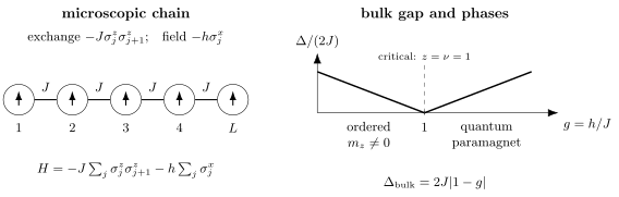
The ferromagnetic one-dimensional chain balances $z$-axis exchange against an $x$-directed field. In the infinite chain with $J>0$ and $g=h/J\ge0$, the bulk quasiparticle gap closes at $g=1$ and reopens in the quantum paramagnet.

Global Spin-Flip Symmetry

Define

$$\mathcal P = \prod_{j=1}^{L} \sigma_j^x.$$

Because operators on different sites commute,

$$\mathcal P^2=I.$$

Conjugation gives

$$\mathcal P \sigma_j^z \mathcal P^{-1} = -\sigma_j^z,$$

and

$$\mathcal P \sigma_j^x \mathcal P^{-1} = \sigma_j^x.$$

Every Ising bond contains two $\sigma^z$ factors, so

$$[\mathcal P,H] = 0.$$

The eigenvalues

$$p=\pm1$$

label two exact parity sectors.

Order Parameter

The longitudinal magnetization per site is

$$M_z = \frac1L \sum_{j=1}^{L} \sigma_j^z.$$

It is odd under the symmetry:

$$\mathcal P M_z\mathcal P^{-1} = -M_z.$$

If a finite-chain eigenstate has definite parity,

$$\mathcal P\lvert\psi_p\rangle = p\lvert\psi_p\rangle,$$

then

$$\langle\psi_p \vert M_z\vert \psi_p\rangle = 0.$$

This exact zero does not rule out an ordered thermodynamic phase.

Finite Symmetry Cats

At $h=0$, parity eigenstates can be formed as

$$\lvert\mathrm{cat}_\pm\rangle = \frac{ \lvert\Uparrow\rangle \pm \lvert\Downarrow\rangle }{\sqrt2}.$$

They satisfy

$$\mathcal P \lvert\mathrm{cat}_\pm\rangle = \pm \lvert\mathrm{cat}_\pm\rangle.$$

Each has

$$\langle M_z\rangle=0,$$

but

$$\langle M_z^2\rangle=1.$$

Long-range two-point correlations and magnetization fluctuations reveal order that the one-point function hides. Their pointwise, squared-order, and finite-size peak criteria are developed in Long-Range Order.

Spontaneous Symmetry Breaking

In the infinite ordered phase, one may select a branch with an infinitesimal longitudinal source. Schematically,

$$m_z = \lim_{\lambda\to0^+} \lim_{L\to\infty} \left\langle M_z \right\rangle_{H-\lambda\sum_j\sigma_j^z}.$$

The order of limits matters. Reversing them keeps a finite system in a parity eigenstate and gives zero.

For the infinite chain,

$$m_z = \begin{cases} (1-g^2)^{1/8}, & 0\le g<1, \\ 0, & g\ge1. \end{cases}$$

The formula refers to a selected symmetry-broken ground state. It is not the expectation value in a finite parity eigenstate.

Ordered and Paramagnetic Regimes

For the infinite ferromagnetic chain:

Regime	Ground-state structure	Long-distance behavior
$0\le g<1$	ordered, two thermodynamic branches	$m_z\ne0$ and long-range $zz$ correlations
$g=1$	scale invariant	gapless with algebraic correlations
$g>1$	quantum paramagnet	unique symmetric bulk phase with exponentially decaying $zz$ correlations

The words ordered and paramagnetic describe thermodynamic regimes. A finite chain has discrete levels and analytic ground-state data away from exact crossings; it does not literally contain two infinite-volume phases.

Correlation Diagnostics

Define

$$C_{zz}(r) = \langle \sigma_j^z \sigma_{j+r}^z \rangle.$$

In a selected ordered ground state,

$$\lim_{r\to\infty} C_{zz}(r) = m_z^2.$$

In the paramagnet,

$$C_{zz}(r) \sim e^{-r/\xi}$$

up to algebraic prefactors. At criticality,

$$C_{zz}(r) \sim \frac{A}{r^{1/4}},$$

where $A$ is nonuniversal while the exponent $1/4$ is universal for the one-dimensional quantum Ising critical point.

Transverse Magnetization

The transverse magnetization is

$$M_x = \frac1L \sum_j \sigma_j^x.$$

For a nondegenerate finite-size ground state, Hellmann–Feynman gives

$$\frac{\partial E_0}{\partial h} = - \left\langle \sum_j\sigma_j^x \right\rangle.$$

Thus

$$\langle M_x\rangle = - \frac1L \frac{\partial E_0}{\partial h}.$$

Unlike $M_z$, the transverse magnetization is even under $\mathcal P$ and can be nonzero in both phases. It approaches one as $g\to\infty$.

Longitudinal Field

Adding

$$H_\lambda = -\lambda \sum_j \sigma_j^z$$

explicitly breaks the global spin-flip symmetry:

$$[\mathcal P,H+H_\lambda] \ne 0 \qquad (\lambda\ne0).$$

The longitudinal field selects one magnetization direction and generally destroys the free-fermion integrability of the nearest-neighbor chain. Results for $\lambda=0$ should not be transferred to $\lambda\ne0$ without a new analysis.

Dual Variables

For an open chain, introduce operators on dual links:

$$\mu_{j+1/2}^x = \sigma_j^z\sigma_{j+1}^z,$$

and

$$\mu_{j+1/2}^z = \prod_{\ell\le j} \sigma_\ell^x.$$

Then neighboring dual strings give

$$\mu_{j-1/2}^z \mu_{j+1/2}^z = \sigma_j^x.$$

The bulk Hamiltonian becomes

$$H \longleftrightarrow - J \sum_j \mu_{j+1/2}^x - h \sum_j \mu_{j-1/2}^z \mu_{j+1/2}^z,$$

up to boundary terms and edge degrees of freedom.

Self-Dual Point

The dual Hamiltonian has the same form with field and exchange interchanged:

$$J \longleftrightarrow h.$$

Equivalently,

$$g \longleftrightarrow \frac1g.$$

The self-dual value is

$$g=1.$$

Duality exchanges the ordered and disordered descriptions. It strongly identifies the candidate transition point, but self-duality alone does not prove that every self-dual model has one unique continuous transition. The exact solution supplies that additional information here.

Exact Solution Strategy

The one-dimensional nearest-neighbor model at zero longitudinal field is integrable. A standard route is:

1. rotate spin axes so the Ising coupling lies along $x$ and the field along $z$;
2. apply a Jordan–Wigner transformation from spins to fermions;
3. separate fermion-parity sectors and impose the corresponding boundary conditions;
4. Fourier transform the quadratic fermion Hamiltonian;
5. perform a Bogoliubov rotation that diagonalizes its pairing terms.

The result is a set of independent fermionic quasiparticles. The mapping is nonlocal, and the periodic spin chain does not become a single periodic fermion problem without parity qualifications.

Adding a generic longitudinal field destroys this free-fermion integrability. The mixed-field chain is therefore a standard finite-size testbed for the eigenstate thermalization hypothesis, provided exact reflection and other symmetries are resolved before comparing eigenstates.

Exact Bulk Dispersion

Let $q=ka$ be dimensionless crystal momentum, with lattice spacing $a$. In the thermodynamic limit,

$$\varepsilon(q) = 2J \sqrt{ 1+g^2-2g\cos q }.$$

Equivalent forms include

$$\varepsilon(q) = 2J \sqrt{ (g-\cos q)^2 + \sin^2q }.$$

The dispersion is nonnegative and periodic in $q$.

The exact finite-chain set of allowed momenta depends on spin boundary conditions and fermion parity. The continuous function above is the bulk result, not a complete finite-size spectrum by itself.

Bulk Gap

For $g\ge0$, the minimum occurs at $q=0$. Therefore

$$\Delta_{\mathrm{bulk}} = \varepsilon(0) = 2J \lvert1-g\rvert.$$

The bulk gap is nonzero for

$$g\ne1$$

and closes at

$$g_c=1.$$

This gap is the quasiparticle mass scale in the infinite system. In the ordered phase it must be distinguished from the exponentially small splitting between finite-size parity partners.

Critical Dispersion

At $g=1$,

$$\varepsilon(q) = 2J \sqrt{ 2-2\cos q }.$$

Using

$$2-2\cos q = 4\sin^2\frac q2,$$

gives

$$\varepsilon(q) = 4J \left| \sin\frac q2 \right|.$$

For $\lvert q\rvert\ll1$,

$$\varepsilon(q) \sim 2J\lvert q\rvert.$$

Restoring $q=ka$, the low-energy velocity is

$$v = \frac{2Ja}{\hbar}.$$

The linear dispersion implies dynamical exponent

$$z=1.$$

Correlation-Length Exponent

Near the transition,

$$\Delta_{\mathrm{bulk}} = 2J \lvert1-g\rvert.$$

Relativistic scaling with $z=1$ gives

$$\Delta \sim \xi^{-1}.$$

Hence

$$\xi \sim \lvert1-g\rvert^{-1},$$

so

$$\nu=1.$$

The model-specific values $z=\nu=1$ agree with the two-dimensional classical Ising universality class. The general meaning and extraction of these exponents belong to Critical Exponents and Scaling.

Exact Ground-State Energy Density

In the thermodynamic limit, the ground-state energy per site is

$$e_0(g) = - \frac12 \int_{-\pi}^{\pi} \frac{dq}{2\pi} \, \varepsilon(q).$$

Equivalently,

$$e_0(g) = - \frac{J}{\pi} \int_0^\pi dq\, \sqrt{ 1+g^2-2g\cos q }.$$

The limiting checks are

$$e_0(0)=-J,$$

and

$$e_0(g) \sim -Jg = -h \qquad (g\to\infty).$$

The energy itself remains continuous at $g=1$, while higher derivatives reveal the critical nonanalyticity.

Exact Critical Data

For the infinite chain in the convention used here:

Quantity	Exact critical behavior
critical coupling	$g_c=1$
bulk gap	$\Delta=2J\lvert1-g\rvert$
dynamical exponent	$z=1$
correlation-length exponent	$\nu=1$
order-parameter exponent	$\beta_{\mathrm{op}}=1/8$
critical $zz$ exponent	$\eta=1/4$
conformal central charge	$c=1/2$

These values characterize the clean nearest-neighbor chain. Disorder, long-range interactions, dissipation, or additional fields can change the universality class or remove integrability.

Quasiparticles and Physical Excitations

At $g=0$, the bulk formula gives

$$\varepsilon(q)=2J.$$

This is the energy assigned to one fermionic domain-wall quasiparticle in the infinite-chain description. On a periodic spin ring, domain walls occur in pairs, so a physical excitation within a fixed boundary and parity sector can cost $4J$ at $h=0$.

The distinction between a quasiparticle dispersion and the lowest allowed finite-size many-body excitation is essential. Boundary conditions and global constraints decide which quasiparticle occupations represent physical spin states.

Finite-Size Parity Sectors

Because

$$[\mathcal P,H]=0,$$

the Hilbert space splits as

$$\mathcal H = \mathcal H_+ \oplus \mathcal H_-.$$

For $L\ge1$,

$$\dim\mathcal H_+ = \dim\mathcal H_- = 2^{L-1}.$$

Exact diagonalization can work in either parity block. For a periodic uniform chain, translation and reflection can provide further block structure.

The Jordan–Wigner transform ties fermion boundary conditions to $\mathcal P$. Ignoring that relation can produce incorrect finite-size momentum grids or an unphysical ground-state sector.

Three Different Gaps

Finite Ising-chain discussions often mix three quantities.

1. Symmetry-partner splitting: the energy difference between the lowest even and odd parity states. It is exponentially small in $L$ throughout the ordered phase.
2. Bulk excitation gap: the cost of a local quasiparticle excitation. It remains finite away from $g=1$.
3. Finite-size critical gap: at $g=1$, low levels scale as $v/L$ with coefficients fixed by boundary conditions and operator sectors.

A numerical plot labeled only “the gap” is incomplete.

Scaling of the Finite Critical Gap

At $g=1$, the dispersion is linear:

$$\varepsilon(k) \sim \hbar v\lvert k\rvert.$$

Finite length quantizes momenta in steps of order

$$\Delta k \sim \frac1L.$$

Therefore a low critical excitation scales as

$$\Delta_L \propto \frac{\hbar v}{L}.$$

The proportionality constant depends on open versus periodic boundaries and on the parity or conformal sector. The robust statement is the power

$$\Delta_L\propto L^{-1},$$

consistent with $z=1$.

Exact Two-Site Open Chain

For $L=2$ with one exchange bond,

$$H_2 = -J\sigma_1^z\sigma_2^z - h \left( \sigma_1^x+\sigma_2^x \right).$$

Define parity-even states

$$\lvert\phi_+\rangle = \frac{ \lvert\uparrow\uparrow\rangle + \lvert\downarrow\downarrow\rangle }{\sqrt2},$$

and

$$\lvert\psi_+\rangle = \frac{ \lvert\uparrow\downarrow\rangle + \lvert\downarrow\uparrow\rangle }{\sqrt2}.$$

The even block is

$$H_+ = \begin{pmatrix} -J&-2h\\ -2h&J \end{pmatrix}.$$

Its energies are

$$E_\pm^{(+)} = \pm \sqrt{ J^2+4h^2 }.$$

Odd Two-Site States

The parity-odd states are

$$\lvert\phi_-\rangle = \frac{ \lvert\uparrow\uparrow\rangle - \lvert\downarrow\downarrow\rangle }{\sqrt2},$$

and

$$\lvert\psi_-\rangle = \frac{ \lvert\uparrow\downarrow\rangle - \lvert\downarrow\uparrow\rangle }{\sqrt2}.$$

The transverse-field sum annihilates both states, so

$$E_{\phi_-}=-J, \qquad E_{\psi_-}=J.$$

For $h>0$, the ground state is even with energy

$$E_0 = - \sqrt{ J^2+4h^2 }.$$

This dimer is a finite analytic crossover, not a phase transition.

Two-Site Ground State

Write

$$\tan\vartheta = \frac{2h}{J}, \qquad 0\le\vartheta<\frac{\pi}{2}.$$

The normalized ground state is

$$\lvert\Omega_2\rangle = \cos\frac{\vartheta}{2} \lvert\phi_+\rangle + \sin\frac{\vartheta}{2} \lvert\psi_+\rangle.$$

At $h=0$, this is the even ferromagnetic cat $\lvert\phi_+\rangle$. As $h/J\to\infty$,

$$\lvert\Omega_2\rangle \longrightarrow \lvert+x,+x\rangle.$$

The dimer makes the finite-size interpolation explicit: the exact symmetric ground state evolves smoothly between two limits.

Two-Site Entanglement

Tracing out either spin gives two eigenvalues

$$\lambda_\pm = \frac12 \left( 1 \pm \sin\vartheta \right),$$

where

$$\sin\vartheta = \frac{2h}{ \sqrt{J^2+4h^2} }.$$

The one-spin entanglement entropy is

$$S_1 = - \sum_{\alpha=\pm} \lambda_\alpha \ln\lambda_\alpha.$$

At $h=0$, the even cat has

$$S_1=\ln2.$$

At $h/J\to\infty$, the product paramagnet has

$$S_1\to0.$$

The entropy $\ln2$ at $h=0$ belongs to the finite parity cat. Either selected broken product state has zero bipartite entanglement.

Entanglement Away from Criticality

Both phases are gapped away from $g=1$. In one dimension, a ground-state interval entropy approaches a size-independent constant once the interval is much larger than the correlation length, subject to boundary and cat-state contributions.

Near criticality, the saturation value grows logarithmically with the correlation length. For a single cut in an infinite gapped chain,

$$S \sim \frac{c}{6} \ln\frac{\xi}{a_0} + \text{constant},$$

for the standard conformal scaling geometry, with

$$c=\frac12.$$

The microscopic cutoff $a_0$ and additive constant are nonuniversal.

Critical Entanglement

For a periodic critical chain of length $L$, the ground-state entropy of an interval of $\ell$ consecutive sites has the conformal form

$$\begin{aligned} S(\ell,L) ={}& \frac{c}{3} \ln \left[ \frac{L}{\pi a_0} \sin \left( \frac{\pi\ell}{L} \right) \right] \\ &+ s_1 + o(1), \end{aligned}$$

with

$$c=\frac12.$$

For an interval adjacent to an open boundary, the logarithmic coefficient becomes $c/6$, with boundary-dependent constants. The general entropy definitions and area-law context live in Entanglement Entropy in Many-Body Systems. Geometry-correct estimators and the $c=1/2$ finite-entanglement benchmark are developed in Entanglement and Criticality.

Critical Continuum Theory

At $g=1$, the low-energy theory is described by a massless Majorana field with central charge

$$c=\frac12.$$

Detuning $g-1$ generates a mass whose magnitude is proportional to the bulk gap. The relativistic continuum description is emergent: the microscopic spin chain has a lattice, a preferred time coordinate, and no fundamental Lorentz symmetry.

The broader operator-to-field and scaling bridge is developed in Why Many-Body QM Leads to QFT.

Quantum-to-Classical Mapping

A Trotter decomposition represents the $d$-dimensional quantum Ising partition function as an anisotropic classical Ising model in $d+1$ Euclidean dimensions. For the chain, the zero-temperature critical exponents match those of the two-dimensional classical Ising model.

This correspondence explains the exponent values, but it is not a statement that a finite quantum chain is literally a two-dimensional magnet. Imaginary time, anisotropic couplings, limits, and observable dictionaries must be handled explicitly. The general mapping belongs to Quantum Phase Transitions, Universality owns the class-matching criteria, and Critical Exponents and Scaling owns the exact Ising exponent check, dynamic exponent, correction terms, and finite-size collapse.

Finite Temperature in One Dimension

The ordered and paramagnetic regimes above are zero-temperature phases. For finite-range interactions in one spatial dimension, the clean chain has no nonzero-temperature Ising ordering transition. Any $T>0$ gives a finite density of thermally excited domain walls and a finite longitudinal correlation length.

There can still be broad low-temperature crossover regimes controlled by the nearby zero-temperature critical point. A crossover is not a finite-temperature phase boundary. Finite-Temperature Phase Transitions states the thermodynamic and finite-size criteria behind that distinction.

Sparse-Matrix Representation

In the $\sigma^z$ product basis, the exchange energy is diagonal:

$$\langle\mathbf s\vert H_J\vert\mathbf s\rangle = -J \sum_{\langle j,j+1\rangle} s_js_{j+1}.$$

The field connects a configuration only to the $L$ configurations obtained by flipping one bit:

$$\langle \mathbf s^{(j)} \vert H_h\vert \mathbf s \rangle = -h.$$

Thus each matrix row has at most one diagonal contribution and $L$ one-spin-flip entries before symmetry reduction. The matrix dimension is $2^L$, but the number of nonzero entries per row grows only linearly with $L$.

This structure makes the chain a standard benchmark for Sparse Matrices, Krylov methods, and matrix-free Hamiltonian actions. The MB-B001 and MB-B009 contracts in Benchmark Problems fix small-chain spectra, trace moments, and the exact critical open-chain gap sequence.

Exact-Diagonalization Workflow

For a finite chain:

1. choose open or periodic bonds;
2. fix the Pauli and coupling convention;
3. encode each $\sigma^z$ configuration as an $L$-bit integer;
4. add the diagonal exchange energy;
5. generate each transverse-field neighbor with one bit flip;
6. block by parity and, when available, translation or reflection;
7. compute several low levels in both parity sectors;
8. label the symmetry-partner and bulk gaps separately;
9. evaluate $M_z^2$, correlations, and entanglement;
10. repeat across $L$ before making a thermodynamic claim.

Finite-Size Checks

Reliable checks include:

• at $h=0$, reproduce the classical configuration energies and exact ferromagnetic degeneracy;
• at $J=0$, obtain the product-state ladder with level spacing $2h$;
• verify $[\mathcal P,H]=0$ numerically;
• confirm equal parity-block dimensions;
• compare the $L=2$ spectrum with the analytic result;
• verify that the critical low gap scales approximately as $L^{-1}$;
• distinguish open-chain edge effects from periodic bulk behavior;
• check that increasing $L$ sharpens, rather than invents, critical signatures.

Experimental and Effective Uses

The model can describe actual magnetic moments only when the physical anisotropy and field coupling justify the pseudospin Hamiltonian. It can also describe effective two-level variables in atomic, molecular, optical, superconducting, or programmable systems.

The symbol $\boldsymbol\sigma$ may represent a true spin, a crystal-field doublet, two charge configurations, or another qubit-like degree of freedom. The $\mathbb Z_2$ operation and measured magnetization must be interpreted in that physical encoding.

Agreement with an Ising Hamiltonian over one energy range does not prove that longer-range couplings, longitudinal fields, decoherence, or leakage are absent.

Extensions and Loss of Integrability

Common extensions include:

• a longitudinal field;
• next-nearest-neighbor or long-range Ising exchange;
• spatially varying $J_j$ or $h_j$;
• coupling to a bath;
• time-dependent driving;
• additional $xx$, $yy$, or Heisenberg exchange;
• higher-dimensional lattices.

Most such extensions are not diagonalized by the free-fermion method used for the clean chain. Some retain other special structures, but exact solvability is exceptional and must be demonstrated.

Common Mistakes

• Confusing the diagonal $h=0$ quantum Hamiltonian with every classical Ising statistical problem.
• Forgetting whether $\sigma^\alpha$ or $s^\alpha=\sigma^\alpha/2$ appears in the Hamiltonian.
• Quoting $g_c=1$ without stating the coupling normalization.
• Treating finite-chain $\langle M_z\rangle=0$ as evidence against thermodynamic order.
• Calling the exponentially small parity splitting the bulk gap.
• Using the bulk dispersion with an arbitrary finite momentum grid and ignoring parity.
• Forgetting that periodic domain walls occur in pairs.
• Applying the exact free-fermion solution after adding a longitudinal field.
• Interpreting the finite dimer crossover as a phase transition.
• Comparing open and periodic spectra without correcting the bond count.
• Treating the critical Majorana field as a fundamental relativistic particle.
• Inferring a universal entanglement coefficient without specifying boundary geometry and logarithm convention.

Quick Reference

Item	Result for the clean ferromagnetic chain
Hamiltonian	$-J\sum_j\sigma_j^z\sigma_{j+1}^z-h\sum_j\sigma_j^x$
dimensionless coupling	$g=h/J$
symmetry	$\mathcal P=\prod_j\sigma_j^x$
order parameter	$M_z=L^{-1}\sum_j\sigma_j^z$
critical point	$g_c=1$
bulk dispersion	$2J\sqrt{1+g^2-2g\cos q}$
bulk gap	$2J\lvert1-g\rvert$
selected-state magnetization	$(1-g^2)^{1/8}$ for $g<1$
critical data	$z=\nu=1$, $\beta_{\mathrm{op}}=1/8$, $c=1/2$

Summary

The transverse-field Ising chain is quantum because its exchange and field terms do not commute. Exchange suppresses domain walls and favors two $z$-ordered branches; the transverse field flips spins and ultimately favors an $x$-polarized paramagnet. Their competition produces a continuous transition at $h=J$ in the stated Pauli-matrix convention.

After a ground-state quench, the same Bogoliubov sectors make the model an exact benchmark for Loschmidt-rate dynamical phase transitions: an equally populated critical momentum can generate Fisher-zero crossings and nonanalytic return-rate cusps.

The exact one-dimensional solution gives a fermionic quasiparticle gap $2J\lvert1-h/J\rvert$. Finite chains add essential structure: parity eigenstates have zero longitudinal magnetization, ordered parity partners split exponentially, physical domain walls obey boundary constraints, and critical gaps scale as $L^{-1}$. Entanglement distinguishes finite symmetry cats, gapped product-like regimes, and the $c=1/2$ critical point.

Exercises

Exercise 1: Noncommuting terms and conserved parity

For

$$H = -J \sum_j \sigma_j^z\sigma_{j+1}^z - h \sum_j \sigma_j^x,$$

show that the exchange and field parts do not commute, but that

$$\mathcal P = \prod_j\sigma_j^x$$

commutes with $H$.

Solution

On a shared site,

$$[ \sigma_j^z\sigma_{j+1}^z, \sigma_j^x ] = 2i \sigma_j^y\sigma_{j+1}^z \ne0.$$

Thus $[H_J,H_h]\ne0$ when both couplings are present.

For parity,

$$\mathcal P\sigma_j^z\mathcal P^{-1} = -\sigma_j^z,$$

so a bond transforms as

$$\mathcal P \sigma_j^z\sigma_{j+1}^z \mathcal P^{-1} = \sigma_j^z\sigma_{j+1}^z.$$

Every $\sigma_j^x$ also commutes with the product of all $\sigma_\ell^x$. Hence

$$[\mathcal P,H]=0.$$

Exercise 2: Domain-wall counting

At $h=0$ and $J>0$, express the energy of a configuration in terms of its number of domain walls. Why must a periodic chain have an even number?

Solution

For each bond,

$$-Js_js_{j+1} = -J + 2J \frac{1-s_js_{j+1}}{2}.$$

Therefore

$$E = E_{\mathrm F} + 2J N_{\mathrm{dw}},$$

where $E_{\mathrm F}=-(L-1)J$ for an open chain and $E_{\mathrm F}=-LJ$ for a periodic chain.

On a ring, every change from $+1$ to $-1$ must be followed somewhere by a change from $-1$ back to $+1$ before returning to the initial site. Domain walls therefore occur in pairs, so $N_{\mathrm{dw}}$ is even.

Exercise 3: Exact two-site spectrum

Diagonalize the open two-site Hamiltonian

$$H_2 = -J\sigma_1^z\sigma_2^z - h \left( \sigma_1^x+\sigma_2^x \right)$$

by parity.

Solution

In the even basis

$$\left\{ \lvert\phi_+\rangle, \lvert\psi_+\rangle \right\},$$

the matrix is

$$H_+ = \begin{pmatrix} -J&-2h\\ -2h&J \end{pmatrix}.$$

Its eigenvalues are

$$E_\pm^{(+)} = \pm \sqrt{J^2+4h^2}.$$

In the odd basis

$$\left\{ \lvert\phi_-\rangle, \lvert\psi_-\rangle \right\},$$

the field term vanishes and the energies are

$$E_{\phi_-}=-J, \qquad E_{\psi_-}=J.$$

Thus the full spectrum is

$$\left\{ - \sqrt{J^2+4h^2}, -J, J, \sqrt{J^2+4h^2} \right\}.$$

Exercise 4: Duality

Using

$$\mu_{j+1/2}^x = \sigma_j^z\sigma_{j+1}^z,$$

and

$$\mu_{j+1/2}^z = \prod_{\ell\le j} \sigma_\ell^x,$$

show that the bulk Hamiltonian exchanges $J$ and $h$ under duality.

Solution

The Ising bond is directly

$$\sigma_j^z\sigma_{j+1}^z = \mu_{j+1/2}^x.$$

Neighboring strings cancel except at site $j$:

$$\begin{aligned} \mu_{j-1/2}^z \mu_{j+1/2}^z &= \left( \prod_{\ell\le j-1}\sigma_\ell^x \right) \left( \prod_{\ell\le j}\sigma_\ell^x \right) \\ &= \sigma_j^x. \end{aligned}$$

Hence the bulk terms become

$$H \longleftrightarrow - J \sum_j\mu_{j+1/2}^x - h \sum_j \mu_{j-1/2}^z \mu_{j+1/2}^z.$$

This has the same structure with field and exchange exchanged, up to boundary terms. Therefore $g=h/J$ maps to $1/g$, and the self-dual value is $g=1$.

Exercise 5: Gap and critical exponents

Starting from

$$\varepsilon(q) = 2J \sqrt{ 1+g^2-2g\cos q },$$

find the bulk gap for $g\ge0$ and determine $z$ and $\nu$.

Solution

The expression under the square root is minimized at $q=0$, so

$$\Delta = \varepsilon(0) = 2J\lvert1-g\rvert.$$

At $g=1$,

$$\varepsilon(q) = 4J \left| \sin\frac q2 \right| \sim 2J\lvert q\rvert.$$

The critical dispersion is linear, giving

$$z=1.$$

Near criticality,

$$\Delta \propto \lvert1-g\rvert.$$

Since $\Delta\sim\xi^{-z}$ and $z=1$,

$$\xi \sim \lvert1-g\rvert^{-1},$$

so

$$\nu=1.$$

Exercise 6: Hidden order in a parity cat

For

$$\lvert\mathrm{cat}_+\rangle = \frac{ \lvert\Uparrow\rangle + \lvert\Downarrow\rangle }{\sqrt2},$$

compute $\langle M_z\rangle$, $\langle M_z^2\rangle$, and $\langle\sigma_i^z\sigma_j^z\rangle$.

Solution

The two branches have opposite magnetization:

$$M_z\lvert\Uparrow\rangle = \lvert\Uparrow\rangle, \qquad M_z\lvert\Downarrow\rangle = -\lvert\Downarrow\rangle.$$

Their equal superposition therefore gives

$$\langle M_z\rangle=0.$$

Both branches are eigenstates of $M_z^2$ with eigenvalue one, so

$$\langle M_z^2\rangle=1.$$

For any distinct or equal sites,

$$\sigma_i^z\sigma_j^z$$

has eigenvalue $+1$ on both branches. Cross terms vanish, and

$$\langle \sigma_i^z\sigma_j^z \rangle = 1.$$

The one-point order parameter vanishes by parity, while fluctuations and long-range correlations retain the ordered structure.

Exercise 7: Cat-state entanglement

Partition a nontrivial chain into regions $A$ and $B$. Compare the entanglement entropy of $\lvert\Uparrow\rangle$, $\lvert\mathrm{cat}_+\rangle$, and $\lvert+x\rangle^{\otimes L}$.

Solution

Both product states factor across the cut:

$$\lvert\Uparrow\rangle = \lvert\Uparrow\rangle_A \otimes \lvert\Uparrow\rangle_B,$$

and

$$\lvert+x\rangle^{\otimes L} = \lvert+x\rangle_A \otimes \lvert+x\rangle_B.$$

Their entanglement entropies are zero.

For the cat state,

$$\lvert\mathrm{cat}_+\rangle = \frac1{\sqrt2} \left( \lvert\Uparrow\rangle_A \lvert\Uparrow\rangle_B + \lvert\Downarrow\rangle_A \lvert\Downarrow\rangle_B \right).$$

The two branch states are orthogonal in both nonempty regions. The reduced density matrix has eigenvalues $1/2$ and $1/2$, so

$$S_A = -2 \left( \frac12\ln\frac12 \right) = \ln2.$$

This is global cat entanglement, not the same as the scale-dependent critical entanglement at $g=1$.

Exercise 8: Sparse connectivity and symmetry blocks

In the $\sigma^z$ basis for $L$ sites, how many configurations can the transverse field connect to a given basis configuration? What are the parity-block dimensions?

Solution

Each term $\sigma_j^x$ flips exactly one site. There are $L$ choices, so the field connects a basis configuration to $L$ distinct one-bit-flipped configurations.

The exchange term is diagonal. Thus a row has one diagonal entry and at most $L$ off-diagonal field entries.

The parity operator has eigenvalues $\pm1$. Multiplying any $\sigma^z$ configuration by the global spin flip pairs it with a distinct reversed configuration. Symmetric and antisymmetric combinations give one state in each sector per pair. Since there are $2^L$ configurations,

$$\dim\mathcal H_+ = \dim\mathcal H_- = 2^{L-1}.$$

References

• S. Sachdev, Quantum Phase Transitions, 2nd ed., Cambridge University Press, 2011.
• P. Pfeuty, “The One-Dimensional Ising Model with a Transverse Field”, Annals of Physics 57, 79–90, 1970.
• E. Lieb, T. Schultz, and D. Mattis, “Two Soluble Models of an Antiferromagnetic Chain”, Annals of Physics 16, 407–466, 1961.
• E. Barouch and B. M. McCoy, “Statistical Mechanics of the XY Model. II. Spin-Correlation Functions”, Physical Review A 3, 786–804, 1971.
• B. K. Chakrabarti, A. Dutta, and P. Sen, Quantum Ising Phases and Transitions in Transverse Ising Models, Springer, 1996.
• A. Dutta et al., Quantum Phase Transitions in Transverse Field Spin Models, Cambridge University Press, 2015.
• G. Vidal, J. I. Latorre, E. Rico, and A. Kitaev, “Entanglement in Quantum Critical Phenomena”, Physical Review Letters 90, 227902, 2003.
• P. Calabrese and J. Cardy, “Entanglement Entropy and Quantum Field Theory”, Journal of Statistical Mechanics P06002, 2004.
• J. B. Kogut, “An Introduction to Lattice Gauge Theory and Spin Systems”, Reviews of Modern Physics 51, 659–713, 1979.
• S. Suzuki, J.-i. Inoue, and B. K. Chakrabarti, Quantum Ising Phases and Transitions in Transverse Ising Models, 2nd ed., Springer, 2013.