t–J Model Preview

The t–J model describes spin-$1/2$ fermions moving through a lattice under the strict constraint that no site may be doubly occupied. Its standard nearest-neighbor Hamiltonian is

$$\begin{aligned} H_{tJ} ={}& -t \sum_{\langle i,j\rangle,\sigma} \left( \widetilde c_{i\sigma}^\dagger \widetilde c_{j\sigma} + \widetilde c_{j\sigma}^\dagger \widetilde c_{i\sigma} \right) \\ &+ J \sum_{\langle i,j\rangle} \left( \mathbf s_i\cdot\mathbf s_j - \frac14\widetilde n_i\widetilde n_j \right). \end{aligned}$$

The projected operators $\widetilde c_{i\sigma}$ move an electron only when the destination is empty. The exchange term rewards a spin singlet on an occupied bond. These processes compete: hole motion tends to rearrange the spin background, while antiferromagnetic exchange favors local singlet correlations.

For the single-band repulsive Hubbard model with $U\gg\lvert t\rvert$, the leading exchange is

$$J = \frac{4\lvert t\rvert^2}{U} >0.$$

The relation is controlled only within a specified strong-coupling expansion. A phenomenological t–J model may treat $t$, $J$, longer-range hopping, and additional interactions as independent effective parameters.

Canonical Scope

This page is the canonical home for the minimal t–J model as a constrained lattice model: its local Hilbert space, projected operators, Hamiltonian conventions, scale hierarchy, half-filled limit, doped interpretation, diagnostics, and limitations. It is an advanced bridge rather than a full survey of doped Mott phases.

The parent fermionic Hamiltonian lives in Hubbard Model. The controlled elimination of virtual doublon states, including the projector formula and three-site terms, is derived in Effective Hamiltonians in Many-Body Systems. Heisenberg Model owns the spin-only problem reached at half filling.

Detailed material-specific reductions, cuprate band structures, experimental phase diagrams, and claims about high-temperature superconductivity belong in the materials-facing t–J Model article. This page explains why the model is relevant to those questions without presenting any proposed phase or mechanism as settled.

Constrained Local Hilbert Space

An unconstrained spinful fermion site has four states,

$$\lvert0\rangle_i, \qquad \lvert\uparrow\rangle_i, \qquad \lvert\downarrow\rangle_i, \qquad \lvert\uparrow\downarrow\rangle_i.$$

The t–J site retains only

$$\mathcal H_i^{(tJ)} = \operatorname{span} \left\{ \lvert0\rangle_i, \lvert\uparrow\rangle_i, \lvert\downarrow\rangle_i \right\}.$$

The doublon $\lvert\uparrow\downarrow\rangle_i$ is not a high-energy state still present in the model. It has been removed from the low-energy Hilbert space.

Define the global no-double-occupancy projector

$$P = \prod_i \left( 1-n_{i\uparrow}n_{i\downarrow} \right).$$

Physical states satisfy

$$P\lvert\Psi\rangle = \lvert\Psi\rangle.$$

The constraint can also be written locally as

$$n_{i\uparrow}n_{i\downarrow} =0$$

on the physical subspace.

Hilbert-space dimension

For $L$ sites, $N_\uparrow$ up-spin electrons, and $N_\downarrow$ down-spin electrons with $N_\uparrow+N_\downarrow\le L$, the constrained basis has dimension

$$\dim\mathcal H_{L,N_\uparrow,N_\downarrow}^{(tJ)} = \binom{L}{N_\uparrow} \binom{L-N_\uparrow}{N_\downarrow}.$$

If only the total electron number $N_e$ is fixed, summing over spin assignments gives

$$\dim\mathcal H_{L,N_e}^{(tJ)} = \binom{L}{N_e}2^{N_e}.$$

The full constrained space has dimension $3^L$, smaller than the Hubbard space $4^L$ but still exponentially large.

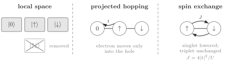
The t–J model retains the empty and singly occupied states while removing the doublon. Projected hopping moves charge at scale $t$ only into an empty site. Exchange acts on two occupied sites at scale $J$ and lowers the spin singlet relative to the triplet.

Projected Fermion Operators

The projected annihilation and creation operators are

$$\begin{aligned} \widetilde c_{i\sigma} &= Pc_{i\sigma}P = c_{i\sigma} \left( 1-n_{i\bar\sigma} \right), \\ \widetilde c_{i\sigma}^\dagger &= Pc_{i\sigma}^\dagger P = \left( 1-n_{i\bar\sigma} \right) c_{i\sigma}^\dagger. \end{aligned}$$

Here $\bar\sigma$ denotes the spin opposite to $\sigma$. Acting on the local states,

$$\begin{aligned} \widetilde c_{i\uparrow}^\dagger \lvert0\rangle_i &= \lvert\uparrow\rangle_i, \\ \widetilde c_{i\uparrow}^\dagger \lvert\downarrow\rangle_i &=0. \end{aligned}$$

The second line is the constraint in action: creating an up electron on a down-occupied site would make a forbidden doublon.

The algebra is not canonical

Projection changes the local operator algebra. For one spin component,

$$\left\{ \widetilde c_{i\sigma}, \widetilde c_{i\sigma}^\dagger \right\} = 1-n_{i\bar\sigma},$$

not the identity. Matrix elements therefore depend explicitly on the occupation of the opposite-spin state.

It is unsafe to manipulate $\widetilde c$ as though it were an ordinary canonical fermion and impose the constraint only at the end. The constraint and algebra are coupled.

Hubbard Operators

An exact local notation uses Hubbard operators

$$X_i^{ab} = \lvert a\rangle_i {}_i\!\langle b\rvert, \qquad a,b\in\{0,\uparrow,\downarrow\}.$$

They satisfy

$$X_i^{ab}X_i^{cd} = \delta_{bc}X_i^{ad}$$

and the completeness relation

$$X_i^{00} +X_i^{\uparrow\uparrow} +X_i^{\downarrow\downarrow} =I_i.$$

Projected fermions become

$$\widetilde c_{i\sigma} = X_i^{0\sigma}, \qquad \widetilde c_{i\sigma}^\dagger = X_i^{\sigma0}.$$

The local density and spin operators are

$$\begin{aligned} \widetilde n_i &= X_i^{\uparrow\uparrow} +X_i^{\downarrow\downarrow}, \\ s_i^z &= \frac12 \left( X_i^{\uparrow\uparrow} -X_i^{\downarrow\downarrow} \right), \\ s_i^+ &= X_i^{\uparrow\downarrow}, \qquad s_i^- = X_i^{\downarrow\uparrow}. \end{aligned}$$

This representation enforces the local space exactly. Auxiliary-particle representations can also encode the constraint, but they enlarge the Hilbert space and introduce a gauge redundancy that must be handled rather than ignored.

Standard Hamiltonian

For real nearest-neighbor hopping and isotropic exchange,

$$H_{tJ} = H_t+H_J,$$

where

$$H_t = -t \sum_{\langle i,j\rangle,\sigma} \left( \widetilde c_{i\sigma}^\dagger \widetilde c_{j\sigma} + \mathrm{h.c.} \right),$$

and

$$H_J = J \sum_{\langle i,j\rangle} \left( \mathbf s_i\cdot\mathbf s_j - \frac14 \widetilde n_i\widetilde n_j \right).$$

A grand Hamiltonian adds

$$-\mu \sum_i\widetilde n_i.$$

The local constraint is part of the model definition. Writing the same polynomial with unprojected $c_{i\sigma}$ on the four-state Hubbard space defines a different Hamiltonian.

Why the density term is present

On a bond with one electron at each endpoint,

$$\widetilde n_i\widetilde n_j=1.$$

The spin operator has eigenvalues

$$\mathbf s_i\cdot\mathbf s_j = \begin{cases} -3/4, & \text{singlet},\\ +1/4, & \text{triplet}. \end{cases}$$

Therefore

$$\mathbf s_i\cdot\mathbf s_j - \frac14\widetilde n_i\widetilde n_j = \begin{cases} -1, & \text{singlet},\\ 0, & \text{triplet}. \end{cases}$$

The exchange term lowers an occupied-bond singlet by $J$ and leaves an occupied-bond triplet unchanged. If either endpoint is empty, both the spin and density contributions vanish.

Dropping $-J\widetilde n_i\widetilde n_j/4$ is harmless at exactly one electron per site because it is then a constant per bond. Away from half filling it is dynamical and cannot be discarded without changing the model.

Large-U Hubbard Origin

Begin with the repulsive Hubbard Hamiltonian

$$H_{\mathrm{Hub}} = T+UD,$$

where

$$D = \sum_i n_{i\uparrow}n_{i\downarrow}.$$

Let $P$ project onto $D=0$ and $Q=I-P$. When $U$ is the largest local energy, virtual states in $Q$ can be removed perturbatively. To second order in the nearest-neighbor hopping,

$$H_{\mathrm{eff}} = PTP - \frac1U PTQTP + O\!\left( \frac{t^3}{U^2} \right).$$

The first term is projected hopping. The second contains bond exchange and correlated processes involving three sites.

The complete derivation, including the sign of the energy denominator and the separation of half-filled and doped sectors, is in Effective Hamiltonians in Many-Body Systems. Here the result fixes the interpretation of the model parameters.

Two distinct low-energy scales

The projected hopping survives at order $t$, while exchange arises at order $t^2/U$:

$$\lvert J\rvert \sim \frac{t^2}{U} \ll \lvert t\rvert \ll U.$$

For the simple one-band repulsive model,

$$\frac{J}{\lvert t\rvert} = \frac{4\lvert t\rvert}{U} \ll1.$$

Treating $J/t$ as order unity can define a useful phenomenological t–J model, but it is not the asymptotic large-$U$ limit of this simplest Hubbard parent.

Why Doping Restores First-Order Motion

At half filling within the constrained space, every site contains one electron. Any single hop would place an electron on an occupied site, so

$$PTP=0.$$

Hopping contributes only through virtual excursions to the doublon sector, producing exchange.

With a hole present, an electron can move into the empty site without creating a doublon. Both the initial and final states remain in $P$, and the matrix element survives at order $t$.

Define the hole concentration for $N_e\le L$ by

$$\delta = \frac{N_h}{L} = 1-\frac{N_e}{L}.$$

Then

$$\delta=0$$

is half filling, while $\delta>0$ introduces mobile holes. The standard no-doublon t–J representation is naturally adapted to hole doping. Electron-doped applications require an explicit particle–hole transformation or a correspondingly chosen low-energy representation; they should not be inferred by silently allowing doublons back into the same Hilbert space.

Half-Filled Limit

At half filling,

$$\widetilde n_i=1$$

on every site and the projected hopping vanishes. If $N_b$ is the number of nearest-neighbor bonds,

$$H_{tJ} \longrightarrow J \sum_{\langle i,j\rangle} \mathbf s_i\cdot\mathbf s_j - \frac{J}{4}N_b.$$

The last term is a constant. The dynamical Hamiltonian is therefore the antiferromagnetic Heisenberg model for $J>0$.

This limit is an exact reduction inside the minimal t–J model. The statement that a particular microscopic material reduces to that model still depends on the validity of the preceding scale separation and orbital reduction.

Three-Site Terms

A systematic Hubbard expansion away from half filling produces correlated three-site hopping at the same order $t^2/U$ as $H_J$:

$$H_{\mathrm{eff}} = H_t+H_J+H_{3\mathrm s} + O\!\left( \frac{t^3}{U^2} \right).$$

Schematically, an electron can hop through an occupied intermediate site by visiting a virtual doublon state and then return to the constrained sector on a different bond. The amplitude is of order

$$\frac{t_{ij}t_{jk}}{U}.$$

The commonly named “minimal t–J model” sets $H_{3\mathrm s}=0$. That omission is an additional approximation, not a consequence of no double occupancy. It may be reasonable for a chosen observable and parameter range, but it must be stated.

At half filling, three-site charge motion is blocked and the spin-only reduction is cleaner. At finite doping, omitting $H_{3\mathrm s}$ while retaining every exchange term is not a uniform truncation solely by powers of $t/U$.

Symmetries

For uniform real hopping and isotropic exchange, the standard model has:

• global $U(1)$ charge conservation;
• global $SU(2)$ spin rotation;
• lattice translations and point-group symmetries when the geometry permits;
• time-reversal symmetry, with complex conjugation of orbital amplitudes and reversal of spin;
• the exact local no-double-occupancy constraint.

The total electron number

$$N_e = \sum_i\widetilde n_i$$

commutes with $H_{tJ}$, as does total spin for the isotropic model:

$$\left[ H_{tJ}, \mathbf S_{\mathrm{tot}}^2 \right] =0, \qquad \mathbf S_{\mathrm{tot}} = \sum_i\mathbf s_i.$$

Longer-range hopping, magnetic flux, spin–orbit coupling, anisotropic exchange, disorder, or boundaries reduce this symmetry set in model-specific ways.

Sign and Gauge Conventions

For nearest-neighbor hopping on a bipartite lattice, the sign of $t$ can be reversed by a staggered phase transformation. Once next-neighbor hopping $t'$, triangular loops, or magnetic flux are present, relative signs and loop phases become physical.

The sign of $J$ is independently meaningful. The repulsive single-band Hubbard limit gives

$$J>0,$$

favoring antiferromagnetic singlets. A ferromagnetic $J<0$ defines a different effective model and is not generated by the simple $4t^2/U$ mechanism.

Physical Competition

The t–J model is not a free hole moving through an inert magnet. Every projected hop changes which sites carry spins and can disrupt or rearrange short-range antiferromagnetic correlations. Conversely, the spin background changes the coherent paths available to a hole.

Three tendencies are useful for orientation:

Tendency	Favored by	Diagnostic examples
coherent carrier motion	larger $\lvert t\rvert$ and available holes	kinetic energy, charge stiffness, spectral weight
antiferromagnetic singlets	$J>0$ near half filling	spin structure factor, bond energy
charge clustering or phase separation	sufficiently strong effective attraction in some parameter regimes	density curvature, real-space inhomogeneity

This table is not a universal phase diagram. Dimension, lattice, $J/t$, longer-range hopping, boundary conditions, and omitted terms all matter.

Relation to Strongly Correlated Electrons

The model is a canonical idealization of a doped Mott insulator. It keeps low-energy spin and charge motion but removes explicit doublon excitations whose cost is assumed to be large.

For cuprate materials, a one-band t–J description is itself the endpoint of a material-dependent reduction from copper and oxygen orbitals. The Zhang–Rice construction supplies one influential route by identifying a local low-energy singlet, but its quantitative range depends on orbital energies, hybridization, interactions, and the observable under study.

Realistic effective descriptions may require

$$t', \qquad t'', \qquad H_{3\mathrm s}, \qquad \text{ring exchange},$$

as well as electron–phonon, disorder, interlayer, or multiorbital effects. The minimal model is valuable because it isolates constrained motion and exchange, not because every strongly correlated material is exactly described by two parameters.

The model has played a central role in theories of unconventional superconductivity, pseudogap behavior, magnetic polarons, and spin–charge separation. Those connections are active research programs. The t–J Hamiltonian alone does not constitute a settled derivation of any one material phase diagram or pairing mechanism.

Controlled and Special Limits

Half filling

At $\delta=0$, the model reduces to Heisenberg exchange plus a constant.

Empty lattice

At $N_e=0$, both hopping and exchange annihilate the vacuum.

One electron

With one electron, the exchange term vanishes and projected hopping reduces to an ordinary one-particle tight-binding problem.

Infinite-U one-hole limit

The $U\to\infty$ Hubbard limit gives $J\to0$. Under restrictive lattice-connectivity and hopping-sign assumptions, Nagaoka’s theorem establishes saturated ferromagnetism for a single hole. The theorem is an exact corner case, not a generic finite-doping phase statement.

One-dimensional special points

The one-dimensional model has Bethe-ansatz-solvable supersymmetric points. With the conventional choice $t>0$, the commonly discussed point $J/t=2$ is not the asymptotic large-$U$ Hubbard regime, where $J/t\ll1$. Exact solvability at a special phenomenological ratio should not be confused with the controlled parent-model expansion.

Observables

Hole density

The local hole operator is

$$h_i = 1-\widetilde n_i.$$

Density profiles and correlations

$$C_h(i,j) = \langle h_i h_j\rangle - \langle h_i\rangle \langle h_j\rangle$$

diagnose clustering, repulsion, or spatial inhomogeneity.

Spin correlations

The static spin structure factor can be defined as

$$S(\mathbf q) = \frac1L \sum_{i,j} e^{-i\mathbf q\cdot(\mathbf R_i-\mathbf R_j)} \langle \mathbf s_i\cdot\mathbf s_j \rangle.$$

Near half filling on a square bipartite lattice, weight near $(\pi/a,\pi/a)$ diagnoses antiferromagnetic correlations. A peak on a finite cluster is not by itself proof of spontaneous order.

Projected momentum distribution

The electron momentum distribution uses projected correlators:

$$n_\sigma(\mathbf k) = \frac1L \sum_{i,j} e^{i\mathbf k\cdot(\mathbf R_i-\mathbf R_j)} \left\langle \widetilde c_{i\sigma}^\dagger \widetilde c_{j\sigma} \right\rangle.$$

Projection redistributes spectral weight and prevents a naive free-fermion interpretation of this function.

Singlet pairing correlations

On a bond $ij$, define a projected singlet creator

$$\Delta_{ij}^\dagger = \frac1{\sqrt2} \left( \widetilde c_{i\uparrow}^\dagger \widetilde c_{j\downarrow}^\dagger - \widetilde c_{i\downarrow}^\dagger \widetilde c_{j\uparrow}^\dagger \right).$$

Pair correlations such as

$$\left\langle \Delta_{ij}^\dagger \Delta_{kl} \right\rangle$$

can compare spatial symmetries and decay laws. A negative pair-binding energy or enhanced short-range correlator on one finite cluster is not sufficient to establish bulk superconducting order.

Charge response

Finite-size addition energies, compressibility, Drude weight, and twist sensitivity probe charge motion. They must be extrapolated at fixed density and with declared boundary conditions.

Finite-Size Formulation

At fixed $N_\uparrow$ and $N_\downarrow$, enumerate only configurations with no shared up- and down-spin site. This enforces the constraint before matrix construction and avoids carrying forbidden states with an artificial penalty.

The hopping matrix element between allowed occupation states retains the fermionic sign fixed by the global mode ordering. Projection removes some destinations but does not remove anticommutation signs.

The exchange term can be written as diagonal $s_i^zs_j^z-\widetilde n_i\widetilde n_j/4$ contributions plus spin flips,

$$\frac{J}{2} \left( s_i^+s_j^- + s_i^-s_j^+ \right).$$

This decomposition is useful for sparse exact diagonalization and tensor-network implementations.

Numerical Methods and Difficulties

Exact diagonalization

The constrained basis is smaller than the Hubbard basis, but its exponential growth still restricts clusters. Translation, point-group, total momentum, particle number, and $S^z$ sectors are valuable.

Tensor networks

Matrix-product-state methods are powerful in one dimension and on narrow cylinders. Two-dimensional conclusions require width, bond-dimension, boundary, and truncation analyses.

Quantum Monte Carlo

Mobile fermionic carriers generally reintroduce a sign problem. The absence of doublons does not make the model generically sign-problem free.

Variational projected states

Variational Many-Body States derives the fermionic Gutzwiller operator and distinguishes partial doublon suppression from hard projection. Gutzwiller-projected Slater or paired states satisfy the local constraint and can encode candidate metallic, magnetic, or paired correlations. Variational success compares energies and observables within a chosen family; it does not prove that the family contains the exact phase.

Auxiliary particles

Parton or slave-particle decompositions can separate spin and charge variables at the cost of enlarging the Hilbert space. Their local constraint generates a gauge redundancy. A saddle point that violates the constraint or neglects gauge fluctuations is an approximation, not an exact rewriting of the physical spectrum.

Model Boundaries

The minimal t–J model omits:

• explicit doublon excitations at energy $U$;
• the upper Hubbard band;
• three-site terms unless added;
• longer-range hopping and exchange unless specified;
• orbital and ligand degrees of freedom;
• phonons, disorder, and long-range Coulomb interaction;
• higher-order ring exchange;
• coupling to electromagnetic or dissipative environments.

If a target experiment directly probes energies comparable with $U$, doublon dynamics, charge-transfer excitations, or multiorbital structure, the t–J Hilbert space is too small.

Common Mistakes

Treating projection as a large but finite penalty

The minimal t–J model has no doublon state. Replacing projection by a finite onsite $U$ returns to a Hubbard-type model with additional high-energy dynamics.

Using canonical fermion algebra for projected operators

The relation

$$\{\widetilde c_{i\sigma},\widetilde c_{i\sigma}^\dagger\} = 1-n_{i\bar\sigma}$$

must be respected. Wick factorization and free-fermion manipulations do not carry over unchanged.

Dropping the density part of exchange away from half filling

The term $-J\widetilde n_i\widetilde n_j/4$ is not constant when holes move.

Calling the minimal model the complete second-order Hubbard theory

Three-site terms also occur at order $t^2/U$ away from half filling.

Confusing half filling with a metal

Within the constrained model at one electron per site, projected hopping is blocked. The low-energy dynamics is spin exchange, not an ordinary half-filled band.

Assuming J/t is arbitrary in a claimed large-U derivation

For the simplest parent,

$$\frac{J}{\lvert t\rvert} = \frac{4\lvert t\rvert}{U}$$

in the standard nearest-neighbor convention. An independent $J/\lvert t\rvert$ is a phenomenological extension.

Overclaiming material relevance

Deriving a one-band constrained model requires an orbital reduction in addition to eliminating doublons. Agreement with one observable does not establish universal quantitative validity.

Inferring bulk pairing from one cluster

Finite-size pair correlations, gaps, and binding energies require scaling and comparison with competing orders.

Worked Example: One Occupied Bond

Consider two occupied neighboring sites. The singlet and triplets are

$$\begin{aligned} \lvert s\rangle &= \frac1{\sqrt2} \left( \lvert\uparrow,\downarrow\rangle - \lvert\downarrow,\uparrow\rangle \right), \\ \lvert t_0\rangle &= \frac1{\sqrt2} \left( \lvert\uparrow,\downarrow\rangle + \lvert\downarrow,\uparrow\rangle \right), \\ \lvert t_+\rangle &= \lvert\uparrow,\uparrow\rangle, \qquad \lvert t_-\rangle = \lvert\downarrow,\downarrow\rangle. \end{aligned}$$

Projected hopping annihilates all four states because neither site is empty. Exchange gives

$$H_J\lvert s\rangle = -J\lvert s\rangle,$$

and

$$H_J\lvert t_m\rangle =0.$$

Thus the singlet–triplet splitting is $J$. In the large-$U$ Hubbard dimer, the same low-energy splitting is $4t^2/U+O(t^4/U^3)$.

Worked Example: One Hole on Two Sites

In the one-electron sector, use basis

$$\left\{ \lvert\sigma,0\rangle, \lvert0,\sigma\rangle \right\}.$$

The exchange term vanishes because no bond has two occupied endpoints. The projected hopping matrix is

$$[H_{tJ}]_\sigma = \begin{pmatrix} 0 & -t\\ -t & 0 \end{pmatrix},$$

with eigenvalues

$$E_\pm = \pm t.$$

This elementary sector isolates first-order charge motion without any virtual doublon.

Exercises

Exercise 1: Count the constrained basis

For $L=6$, $N_\uparrow=2$, and $N_\downarrow=2$, compute the constrained Hilbert-space dimension and compare it with the unconstrained fixed-spin Hubbard dimension.

Solution

Choose the two up-spin sites and then choose the two down-spin sites from the remaining four:

$$\dim\mathcal H^{(tJ)} = \binom62\binom42 = 15\times6 =90.$$

Without the no-double-occupancy constraint, up and down sites are chosen independently:

$$\dim\mathcal H^{(\mathrm{Hub})} = \binom62^2 =225.$$

The difference consists of configurations in which at least one site carries both spins.

Exercise 2: Projected anticommutator

Verify $\{\widetilde c_{i\uparrow},\widetilde c_{i\uparrow}^\dagger\}=1-n_{i\downarrow}$ by acting on the three allowed local states.

Solution

On $\lvert0\rangle$, creation followed by annihilation returns the state, while the reverse order vanishes. The anticommutator gives $1$, matching $1-n_\downarrow$.

On $\lvert\uparrow\rangle$, annihilation followed by creation returns the state, so the result is again $1$.

On $\lvert\downarrow\rangle$, projected up-spin creation and annihilation both vanish. The anticommutator gives $0$, while

$$(1-n_\downarrow)\lvert\downarrow\rangle =0.$$

The three states span the local physical space, proving the identity there.

Exercise 3: Bond exchange spectrum

Show that $\mathbf s_i\cdot\mathbf s_j-\widetilde n_i\widetilde n_j/4$ is minus the singlet projector when both sites are occupied.

Solution

For two spins $1/2$,

$$\mathbf s_i\cdot\mathbf s_j = \frac12 \left( \mathbf s_{\mathrm{tot}}^2 - \mathbf s_i^2 - \mathbf s_j^2 \right).$$

The singlet has total spin zero and eigenvalue $-3/4$; each triplet has total spin one and eigenvalue $1/4$. Since $\widetilde n_i\widetilde n_j=1$,

$$\mathbf s_i\cdot\mathbf s_j - \frac14 = \begin{cases} -1, & \text{singlet},\\ 0, & \text{triplet}. \end{cases}$$

That is precisely $-P_s$.

Exercise 4: Hubbard-dimer exchange

The half-filled Hubbard dimer singlet energy is

$$E_s = \frac12 \left( U-\sqrt{U^2+16t^2} \right),$$

while the triplet energy is zero. Expand the splitting at large positive $U$.

Solution

Use

$$\sqrt{U^2+16t^2} = U \sqrt{1+16t^2/U^2} = U+ \frac{8t^2}{U} + O\!\left( \frac{t^4}{U^3} \right).$$

Therefore

$$E_s = -\frac{4t^2}{U} + O\!\left( \frac{t^4}{U^3} \right).$$

The singlet is lower than the triplet by

$$J = \frac{4t^2}{U}$$

to leading order.

Exercise 5: Half-filled reduction

Show explicitly that the minimal t–J Hamiltonian becomes a Heisenberg Hamiltonian plus a constant at one electron per site.

Solution

Every projected hop has an occupied destination and vanishes, so $H_t=0$. Also $\widetilde n_i\widetilde n_j=1$ on every bond. Hence

$$H_{tJ} = J \sum_{\langle i,j\rangle} \mathbf s_i\cdot\mathbf s_j - \frac J4N_b.$$

The second term is a constant for fixed lattice geometry. Removing it leaves the antiferromagnetic Heisenberg model.

Exercise 6: Why three-site terms are not higher order than exchange

An electron hops from site $i$ to $j$, creates a virtual doublon of cost $U$, and then a fermion hops from $j$ to a distinct neighbor $k$. Estimate the amplitude and compare it with $J$.

Solution

Each hop contributes one hopping matrix element, and the virtual state contributes an energy denominator $1/U$. The process therefore has scale

$$\frac{t_{ij}t_{jk}}{U}.$$

For uniform hopping this is $t^2/U$, the same order as

$$J = \frac{4t^2}{U}.$$

The three-site process may have a smaller numerical coefficient or reduced phase space, but it is not suppressed by an additional power of $t/U$ relative to exchange.

Exercise 7: One-hole projected motion

Explain why projected hopping is zero at half filling but nonzero in a basis state containing one hole.

Solution

At half filling every destination of a nearest-neighbor hop is occupied. Moving an electron there would create a doublon, and projection sets the result to zero.

If site $i$ is empty and neighboring site $j$ is singly occupied, then

$$\widetilde c_{i\sigma}^\dagger \widetilde c_{j\sigma}$$

moves the electron from $j$ to $i$. Both configurations satisfy the local constraint, so the matrix element survives at first order in $t$.

Summary

• The t–J model has three local states: empty, spin up, and spin down.
• Projected fermions are noncanonical operators because their algebra depends on opposite-spin occupation.
• Projected hopping moves holes at order $t$; exchange lowers occupied-bond singlets at order $J$.
• The large-$U$ single-band Hubbard relation is $J=4\lvert t\rvert^2/U$.
• At half filling, hopping is blocked and the model reduces to antiferromagnetic Heisenberg exchange plus a constant.
• Away from half filling, three-site correlated hopping also appears at order $t^2/U$ in a systematic Hubbard expansion.
• The minimal model isolates doped-Mott competition but does not by itself establish a material phase diagram or pairing mechanism.

Further Reading

• Hubbard Model
• Heisenberg Model
• Effective Hamiltonians in Many-Body Systems
• Effective Hamiltonians in Quantum Matter
• Fermionic Operators in Many-Body Models
• Occupation-Number Representation
• Lattice Models Overview
• Correlation Functions Overview
• Equal-Time Correlations
• t–J Model in Quantum Matter
• Hubbard Model Reference Card

References

1. K. A. Chao, J. Spałek, and A. M. Oleś, “Canonical Perturbation Expansion of the Hubbard Model,” Physical Review B 18, 3453–3464 (1978), doi:10.1103/PhysRevB.18.3453.
2. Y. Nagaoka, “Ferromagnetism in a Narrow, Almost Half-Filled s Band,” Physical Review 147, 392–405 (1966), doi:10.1103/PhysRev.147.392.
3. P. W. Anderson, “The Resonating Valence Bond State in La2CuO4 and Superconductivity,” Science 235, 1196–1198 (1987), doi:10.1126/science.235.4793.1196.
4. A. H. MacDonald, S. M. Girvin, and D. Yoshioka, “$t/U$ Expansion for the Hubbard Model,” Physical Review B 37, 9753–9756 (1988), doi:10.1103/PhysRevB.37.9753.
5. F. C. Zhang and T. M. Rice, “Effective Hamiltonian for the Superconducting Cu Oxides,” Physical Review B 37, 3759–3761 (1988), doi:10.1103/PhysRevB.37.3759.
6. E. Dagotto, “Correlated Electrons in High-Temperature Superconductors,” Reviews of Modern Physics 66, 763–840 (1994), doi:10.1103/RevModPhys.66.763.
7. M. Imada, A. Fujimori, and Y. Tokura, “Metal-Insulator Transitions,” Reviews of Modern Physics 70, 1039–1263 (1998), doi:10.1103/RevModPhys.70.1039.
8. P. A. Lee, N. Nagaosa, and X.-G. Wen, “Doping a Mott Insulator: Physics of High-Temperature Superconductivity,” Reviews of Modern Physics 78, 17–85 (2006), doi:10.1103/RevModPhys.78.17.
9. B. Edegger, V. N. Muthukumar, and C. Gros, “Gutzwiller–RVB Theory of High-Temperature Superconductivity: Results from Renormalized Mean-Field Theory and Variational Monte Carlo Calculations,” Advances in Physics 56, 927–1033 (2007), doi:10.1080/00018730701627707.
10. P.-A. Bares, G. Blatter, and M. Ogata, “Exact Solution of the t–J Model in One Dimension at $2t=\pm J$: Ground State and Excitation Spectrum,” Physical Review B 44, 130–136 (1991), doi:10.1103/PhysRevB.44.130.