Exact Solutions Preview

An exact solution replaces a many-body eigenproblem by a structure that can be characterized without uncontrolled approximation. That structure might be a set of independent normal modes, coupled Bethe equations for rapidities, a commuting family of transfer matrices, or exact integral equations for thermodynamic functions. These outcomes are exact in different senses and offer very different access to observables.

The phrase does not mean that every answer is elementary, that every correlation function is available in closed form, or that a finite computer calculation proves a model integrable. The main skill is therefore diagnostic: identify what structure closes, what quantities it determines, and what remains difficult even after the model is called solvable.

Purpose and Canonical Scope

This page is a map of exact methods for quantum lattice systems. It owns:

• a working taxonomy of exactness in many-body physics;
• the general free-mode and Bogoliubov routes;
• the logic of coordinate Bethe ansatz and factorized scattering;
• a careful working meaning of quantum integrability;
• the relation among Yang–Baxter structure, transfer matrices, conserved charges, and thermodynamic Bethe ansatz;
• the practical hierarchy from exact spectra to correlation functions and dynamics;
• the reasons exact solvability is exceptional and usually fragile.

It does not repeat model-specific derivations. Jordan–Wigner Transformation owns the spin–fermion dictionary and parity sectors. Transverse-Field Ising Model owns the Ising spectrum and phase physics. The Heisenberg Chain dossier owns the isotropic chain’s compact exact fingerprints, while the XXZ Chain dossier owns the anisotropic model record and interacting-ring benchmark. XXZ Spin Chain owns the explicit anisotropic Bethe equations and phase structure. Spinless Fermion Chains owns the interacting $t$–$V$ chain.

Why the Generic Problem Is Hard

For $L$ sites of local dimension $d$, the unconstrained Hilbert-space dimension is

$$\dim\mathcal H_L=d^L.$$

A generic Hamiltonian is therefore a matrix whose dimension, not merely its number of entries, grows exponentially. Locality makes the operator sparse and symmetries split it into blocks, but neither fact normally changes the exponential asymptotics of a finite-density sector. Scaling of Hilbert Space develops that obstruction in detail.

Exact solvability occurs when the eigenproblem has additional algebraic or scattering structure. The effective data then scale more gently: one-body eigenvectors, quasiparticle occupations, rapidities, root densities, or a hierarchy of commuting charges replace arbitrary vectors in the full tensor-product space.

This reduction is stronger than knowing a few symmetries. Translation, particle number, parity, or total spin can greatly help a calculation, but a finite list of conserved quantities does not usually determine exponentially many eigenstates.

Several Meanings of Exact

The following uses of exact should not be conflated.

Statement	What is exact	What may remain hard
quadratic or free-mode solution	a canonical transformation diagonalizes the full Hamiltonian	nonlocal observables, determinants, asymptotics, boundary sectors
Bethe-ansatz solution	eigenstates and energies are encoded by coupled algebraic or transcendental equations	root classification, completeness, matrix elements, large-size limits
integrable lattice model	an extensive local or quasilocal commuting hierarchy constrains the dynamics	solving the spectral equations and evaluating observables
exact thermodynamics	free energy and related functions obey exact integral or functional equations	analytic solution of those equations and real-time observables
exact finite-size diagonalization	a chosen finite matrix is diagonalized to numerical precision	the thermodynamic limit and any claim of integrability
rigorous theorem or bound	a stated result follows under explicit hypotheses	construction of all eigenstates or experimentally measurable functions

An implicit equation can be an exact answer. If roots $\{\lambda_j\}$ obey equations derived without approximation and an observable is an exact function of those roots, the result is exact even when the roots require numerical solution. Conversely, a high-precision number for $L=20$ is not automatically an exact solution of the model for arbitrary $L$.

Exact does not mean closed form

There is no universally useful requirement that an exact result be expressible through elementary functions. Many central exact results take the form of:

• a determinant or Pfaffian;
• a set of quantization conditions;
• a Fredholm determinant;
• a nonlinear integral equation;
• a convergent form-factor series;
• a recursion or functional relation;
• an asymptotic formula with rigorously controlled errors.

The mathematical representation and the physical question must be stated together.

Exact does not mean universal

An exact formula can depend on:

• open versus periodic boundaries;
• a parity, charge, or magnetization sector;
• the ordering of limits $L\to\infty$, $T\to0$, and $t\to\infty$;
• a particular normalization of rapidity or spectral parameter;
• whether the observable is local in the variables that diagonalize the Hamiltonian.

These are part of the result, not bookkeeping after the fact.

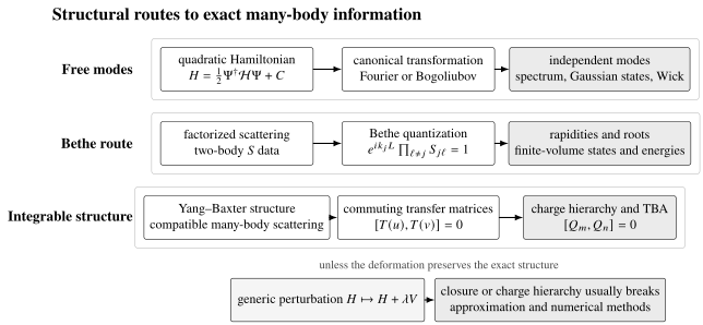
Three related but distinct routes to exact information. Quadratic closure yields independent modes; factorized scattering yields Bethe quantization; Yang–Baxter and transfer-matrix structure produces commuting charges and exact thermodynamic machinery. A generic perturbation usually destroys the relevant closure, although specially constructed deformations can remain integrable.

Route I: Quadratic Hamiltonians

The most transparent exact many-body route is reduction to independent modes. For canonical fermions, a number-conserving quadratic Hamiltonian has the form

$$H = \sum_{i,j=1}^{M} c_i^\dagger h_{ij}c_j +E_0,$$

where $h=h^\dagger$ is an $M\times M$ one-body matrix. Choose a unitary matrix $U$ such that

$$U^\dagger hU = \operatorname{diag} (\varepsilon_1,\ldots,\varepsilon_M).$$

The transformed operators

$$\gamma_\alpha = \sum_i U_{i\alpha}^*c_i$$

obey the same canonical anticommutation relations, and

$$H = \sum_{\alpha=1}^{M} \varepsilon_\alpha \gamma_\alpha^\dagger\gamma_\alpha +E_0.$$

Every many-body eigenstate is labeled by occupations $n_\alpha\in\{0,1\}$:

$$|n_1,\ldots,n_M\rangle = \prod_{\alpha=1}^{M} (\gamma_\alpha^\dagger)^{n_\alpha}|0\rangle,$$ $$E_{\{n\}} = E_0 + \sum_\alpha n_\alpha\varepsilon_\alpha.$$

The exponential list of energies has not disappeared, but it is generated from only $M$ one-body numbers. That compression is the exact structure.

Translation-invariant example

For a periodic chain with hopping $t$ and chemical potential $\mu$,

$$H = -t\sum_j (c_j^\dagger c_{j+1}+c_{j+1}^\dagger c_j) - \mu\sum_j n_j.$$

The discrete Fourier transform gives

$$c_j = \frac{1}{\sqrt L} \sum_k e^{ikj}c_k,$$ $$H = \sum_k \varepsilon(k)c_k^\dagger c_k, \qquad \varepsilon(k) = -2t\cos k-\mu.$$

The allowed $k$ values still depend on the boundary twist. Tight-Binding Model gives the one-body derivation and band interpretation; the Tight-Binding Chain dossier fixes a reproducible chain convention and finite validation targets.

Paired quadratic Hamiltonians

Number conservation is not required. A fermionic quadratic Hamiltonian may contain pairing terms,

$$H = \sum_{i,j} c_i^\dagger A_{ij}c_j + \frac12\sum_{i,j} \left( c_i^\dagger B_{ij}c_j^\dagger + c_j B_{ij}^*c_i \right) +C,$$

with $A=A^\dagger$ and $B=-B^{\mathsf T}$. Introduce the Nambu vector

$$\Psi = \begin{pmatrix} c_1&\cdots&c_M&c_1^\dagger&\cdots&c_M^\dagger \end{pmatrix}^{\mathsf T}.$$

Then

$$H = \frac12\Psi^\dagger \mathcal H_{\mathrm{BdG}} \Psi +C'.$$

A Bogoliubov transformation preserving the canonical anticommutation relations brings the stable problem to

$$H = E_{\mathrm{vac}} + \sum_{a=1}^{M} E_a\eta_a^\dagger\eta_a, \qquad E_a\ge0.$$

This is how the one-dimensional transverse-field Ising and anisotropic XY chains become free quasiparticle theories after the Jordan–Wigner map. The exact spin–fermion dictionary and parity-dependent momentum grids are developed on Jordan–Wigner Transformation.

For bosons, a quadratic Hamiltonian can also be treated by a Bogoliubov transformation, but the transformation is paraunitary rather than unitary in Nambu space. Positivity and dynamical stability must be checked; an algebraic diagonal form with complex frequencies does not describe stable independent oscillators.

Gaussian states and Wick reduction

Ground states and thermal states of stable quadratic Hamiltonians are Gaussian. Their equal-time information is encoded by two-point functions such as

$$C_{ij} = \langle c_i^\dagger c_j\rangle, \qquad F_{ij} = \langle c_i c_j\rangle.$$

Higher products reduce to sums of pairings. For example, in a number-conserving Gaussian state,

$$\langle c_i^\dagger c_j^\dagger c_k c_l \rangle = C_{il}C_{jk} - C_{ik}C_{jl}.$$

This reduction is exact, but a nonlocal spin observable can become a long fermion string and hence a determinant or Pfaffian. A free Hamiltonian does not make every observable a one-body quantity. Wick’s Theorem Preview owns the general contraction rule.

What quadratic solvability buys

Once the canonical transform is known, one can usually obtain:

• the complete finite-size spectrum;
• ground-state and thermal occupations;
• partition functions as products over modes;
• Gaussian correlation matrices;
• unitary dynamics of creation and annihilation operators;
• many entanglement measures from restricted correlation matrices.

The main remaining work lies in boundaries, zero modes, degeneracies, asymptotic evaluation, and observables nonlocal in the diagonal variables.

What makes the route fail

Add a density interaction,

$$V = \sum_{i,j} U_{ij}n_i n_j.$$

After a linear canonical transformation it remains quartic. The Heisenberg equation for $c_i$ now involves cubic operators, whose equations involve higher products. The linear operator algebra no longer closes. Special interacting models may still be Bethe-ansatz integrable, but they are not rendered free by the same one-body diagonalization.

Route II: Coordinate Bethe Ansatz

Bethe ansatz addresses certain interacting one-dimensional systems by exploiting highly constrained scattering. Consider a sector with $M$ particles or spin deviations at ordered positions

$$x_1<x_2<\cdots<x_M.$$

Away from collisions, a coordinate Bethe wavefunction is a superposition of plane waves,

$$\psi(x_1,\ldots,x_M) = \sum_{P\in S_M} A(P) \exp\!\left( i\sum_{a=1}^{M}k_{P_a}x_a \right).$$

The interaction appears in the relations among amplitudes when neighboring particles exchange order. In the simplest scalar case,

$$A(P\circ\tau_a) = S(k_{P_a},k_{P_{a+1}})A(P),$$

where $\tau_a$ swaps adjacent momenta and $S$ is the two-body scattering phase.

Periodic quantization

Move particle $j$ once around a ring of length $L$. It accumulates a propagation phase and scatters through all other particles. Periodicity gives the schematic Bethe equations

$$e^{ik_jL} \prod_{\ell\ne j} S(k_j,k_\ell) = 1, \qquad j=1,\ldots,M.$$

The energy and momentum often remain additive in the rapidity data,

$$E = \sum_{j=1}^{M}\varepsilon(k_j)+E_{\mathrm{ref}},$$ $$P = \sum_{j=1}^{M}p(k_j) \pmod{2\pi}.$$

The model is interacting because the allowed $k_j$ are coupled through $S$. Independent modes would have separate one-body quantization conditions.

Rapidities and Bethe roots

Momentum is not always the natural variable. A rapidity $\lambda$ can rationalize the scattering phase or expose the symmetry of the equations. A common logarithmic structure is

$$L p(\lambda_j) + \sum_{\ell\ne j} \theta(\lambda_j-\lambda_\ell) = 2\pi I_j,$$

where $I_j$ are integers or half-integers fixed by the sector and boundary convention. The solutions $\lambda_j$ are Bethe roots.

Roots need not all remain real. Complex roots can form patterns associated with bound states. The familiar string hypothesis is often an asymptotically powerful classification, but finite-size string deviations, exceptional solutions, and completeness questions must be treated rather than hidden.

Why one dimension helps

In one dimension, particle order can change only through encounters. Exact Bethe structure requires those encounters to factor consistently into two-body scattering, with no diffractive production of new independent momenta. For particles carrying internal labels, different sequences of pairwise exchanges must agree. That consistency leads to the Yang–Baxter equation discussed below.

What the ansatz actually supplies

For a successful model and sector, Bethe ansatz can provide:

1. quantization equations for allowed roots;
2. exact energy and momentum formulas in terms of those roots;
3. eigenvectors through coordinate amplitudes or algebraic creation operators;
4. a path to thermodynamic root densities;
5. in favorable cases, norms, form factors, determinants, and correlation functions.

Each item requires additional work. Writing down Bethe equations is not the same as classifying every admissible solution, proving completeness, or evaluating a dynamical correlator.

The XXZ chain as the canonical example

The uniform nearest-neighbor spin-$1/2$ XXZ chain is interacting for anisotropy $\Delta\ne0$ and nevertheless Bethe-ansatz integrable. Its page derives the coordinate ansatz, gives a rapidity convention, explains the exact phase boundaries, and previews thermodynamic Bethe ansatz. See XXZ Spin Chain for those model-specific statements.

The free XX point, $\Delta=0$, sits at the intersection of the two routes: Jordan–Wigner makes it quadratic, and its Bethe scattering reduces to fermionic exchange. This overlap is a special limit, not evidence that every Bethe-integrable chain is free.

Route III: Quantum Integrability

There is no single context-free definition of quantum integrability accepted for every finite-dimensional, continuum, lattice, and field-theoretic problem. Naively counting commuting operators is too weak: any nondegenerate finite Hamiltonian has spectral projectors that commute with it, but those projectors do not constitute useful local conservation laws.

For translation-invariant quantum lattice models, a productive working criterion is the existence of an extensive family of independent local or quasilocal charges,

$$[H,Q_n]=0, \qquad [Q_m,Q_n]=0,$$

with the number of relevant charges growing with system size. Locality or quasilocality prevents arbitrary spectral projectors from trivializing the definition.

This is a structural criterion, not a slogan. One must specify the family of systems, the boundaries, the locality notion, and the independence of the charges.

A commuting transfer matrix

In many integrable chains, the central object is a transfer matrix $T(u)$ depending on a spectral parameter $u$ and satisfying

$$[T(u),T(v)]=0$$

for all $u$ and $v$. Expanding around a regular point $u_0$ generates commuting charges schematically as

$$Q_{n+1} \propto \left. \frac{d^n}{du^n} \log T(u) \right|_{u=u_0}.$$

For an appropriate normalization, one member of this hierarchy is the Hamiltonian. Higher derivatives produce increasingly extended local or quasilocal conserved quantities.

The phrase transfer matrix originates in classical statistical mechanics. A two-dimensional classical lattice model and a one-dimensional quantum chain can share the same algebraic object; commuting transfer matrices then organize both exact partition functions and quantum conserved charges.

Yang–Baxter consistency

Let $R_{ab}(u)$ act on a pair of auxiliary or local spaces. The Yang–Baxter equation has the schematic form

$$R_{12}(u-v) R_{13}(u-w) R_{23}(v-w) = R_{23}(v-w) R_{13}(u-w) R_{12}(u-v).$$

It states that two different sequences of pairwise rearrangements give the same many-body result. This is the algebraic expression of factorized scattering. Building monodromy and transfer matrices from such an $R$ matrix yields the commuting family above under suitable boundary conditions.

For matrix-valued scattering, this condition is essential: scalar phases commute automatically, whereas internal spin or species labels make exchange order nontrivial.

Integrability is more than symmetry

A global symmetry supplies charges, multiplets, and selection rules. Integrability supplies an extensive hierarchy sufficient to constrain scattering and dynamics far beyond a finite-dimensional Lie algebra. Thus:

• translation invariance does not by itself imply integrability;
• conservation of particle number does not imply integrability;
• global $SU(2)$ symmetry does not imply integrability;
• absence of obvious symmetry does not rule out hidden integrable structure;
• a single extra conserved operator is not normally enough.

Symmetry and integrability can coexist. In the Heisenberg and XXZ chains, familiar spin symmetries organize states while transfer-matrix charges provide the stronger integrable structure.

Integrable does not mean noninteracting

An interacting integrable model can have nontrivial phase shifts, bound states, dressed quasiparticles, and strongly correlated eigenstates. What is absent is generic diffractive many-body scattering, not all scattering. The outgoing rapidity set is constrained by the incoming one, while pairwise phases encode interactions.

Free models are integrable in a broad sense because each mode occupation is conserved. Their charge hierarchy is especially transparent. Interacting Bethe models form a richer class whose quasiparticles are dressed by the state and ensemble.

Thermodynamic Bethe Ansatz Preview

Finite-volume Bethe equations involve a number of roots proportional to $L$ at finite density. In the thermodynamic limit, roots organize into continuous distributions. For species or string type $a$, introduce particle and hole densities $\rho_a(\lambda)$ and $\rho_a^{\mathrm h}(\lambda)$. Logarithmic Bethe equations become coupled constraints of the schematic form

$$\rho_a(\lambda) + \rho_a^{\mathrm h}(\lambda) = a_a(\lambda) - \sum_b (K_{ab}*\rho_b)(\lambda),$$

where

$$(K*f)(\lambda) = \int d\mu\, K(\lambda-\mu)f(\mu).$$

The functions $a_a$ encode bare state densities, while $K_{ab}$ is determined by derivatives of scattering phases. The energy and conserved-charge densities become linear functionals of $\rho_a$.

Entropy of root distributions

Many microscopic Bethe states correspond to the same smooth root densities. Their combinatorial entropy per unit length is

$$s = \sum_a\int d\lambda\, \bigg[ (\rho_a+\rho_a^{\mathrm h}) \ln(\rho_a+\rho_a^{\mathrm h}) - \rho_a\ln\rho_a - \rho_a^{\mathrm h}\ln\rho_a^{\mathrm h} \bigg].$$

Minimizing the free-energy density

$$f=e-Ts-\sum_r\mu_r q_r$$

subject to the Bethe constraints produces nonlinear integral equations for dressed energies. A common schematic form is

$$\epsilon_a = e_a^{\mathrm{bare}} - \sum_r\mu_r q_{r,a} - T\sum_b K_{ab}* \ln\!\left(1+e^{-\epsilon_b/T}\right).$$

Signs, statistics factors, kernels, and particle species are model-dependent. The equation is shown to expose the logic, not as a formula to transplant between models.

Thermodynamic Bethe ansatz can determine exact bulk free energies, susceptibilities, dressed velocities, and phase boundaries. It does not automatically solve finite-size boundaries or real-time correlation functions.

Dressing

Interactions alter the response of a quasiparticle because adding one root rearranges the sea of other roots. A bare one-particle quantity $q_a(\lambda)$ acquires a dressed version satisfying a linear integral equation once the equilibrium filling functions are known. Schematically,

$$q_a^{\mathrm{dr}} = q_a + \sum_b K_{ab}* (\vartheta_b q_b^{\mathrm{dr}}),$$

where $\vartheta_b$ is the occupied fraction of available roots. Dressed energy, momentum, velocity, and charge govern thermodynamics and hydrodynamic transport. This state dependence is one reason an interacting integrable gas is not simply a free gas with renamed particles.

A Hierarchy of Exact Information

Solving one layer does not guarantee the next.

Layer	Typical exact object	Additional challenge
energies	mode sums or Bethe-root formulas	enumerate admissible roots and degeneracies
eigenvectors	Fock states, coordinate waves, algebraic Bethe states	normalization and completeness
thermodynamics	product partition function or TBA equations	solve coupled integral equations and limits
static correlators	Wick determinant, form factors, multiple integrals	sum intermediate states and extract asymptotics
dynamical correlators	spectral or form-factor expansions	analytic continuation and oscillatory sums
finite boundaries	reflection equations or boundary modes	boundary bound states and altered quantization
nonequilibrium evolution	Gaussian propagation or integrable quasiparticle data	initial-state overlaps and long-time limits

This hierarchy explains why an article may correctly call a Hamiltonian exactly solvable while quoting numerical correlation functions. The spectrum can be exact even when the observable requires a difficult resummation. The use of complete charge data and Bethe root densities after a quench belongs to Integrability and Generalized Gibbs Ensembles Preview.

Spectrum versus observables

For an operator $O$, a zero-temperature dynamical structure factor contains matrix elements as well as energies:

$$S_O(q,\omega) = 2\pi \sum_n |\langle n|O_q|0\rangle|^2 \delta(\omega-E_n+E_0).$$

Exact eigenvalues determine the delta-function locations. They do not determine the weights $|\langle n|O_q|0\rangle|^2$. Those form factors can be the harder part of the problem.

Finite volume versus thermodynamic limit

Bethe equations may be exact for every finite $L$, while root-density equations describe only the $L\to\infty$ limit. Conversely, universal finite-size corrections can reveal conformal data not visible in the leading bulk energy. Always label which limit an exact statement concerns.

Why Exact Solvability Is Exceptional

The exact routes above require closure conditions that a generic local perturbation does not respect.

Quadratic closure is nongeneric

For a quadratic Hamiltonian, commutators of $H$ with linear fermion operators remain linear:

$$[H,c_i] = \sum_j (A_{ij}c_j+B_{ij}c_j^\dagger).$$

Quartic interactions generate cubic operators. Their commutators generate still higher products, producing an operator hierarchy rather than a finite-dimensional linear problem.

Factorized scattering is restrictive

In a generic interacting many-body collision, outgoing momenta can explore configurations not obtainable by merely permuting incoming rapidities. This diffraction prevents a wavefunction from being assembled consistently from a fixed set of plane-wave momenta and two-body phases.

For matrix-valued scattering, even nondiffractive two-body data must satisfy Yang–Baxter consistency. That is a set of functional constraints on couplings, not an automatic property of one-dimensionality.

Conserved-charge hierarchies are fragile

Let

$$H(\lambda) = H_0+\lambda V,$$

where $H_0$ has a local conserved charge $Q$. To continue it as

$$Q(\lambda) = Q+\lambda\,\delta Q+O(\lambda^2),$$

conservation at first order requires

$$[H_0,\delta Q] + [V,Q] = 0.$$

For a generic $V$, there is no local or quasilocal $\delta Q$ solving this equation for every charge in the hierarchy. Special deformations can preserve integrability, but they occupy constrained families in coupling space.

Exceptional does not mean physically irrelevant

Exact models are valuable because they:

• provide nonperturbative benchmarks for numerical methods;
• identify phases and transitions that survive nearby perturbations;
• supply controlled starting points for perturbation theory;
• reveal quasiparticles, anomalies, and selection rules hidden in microscopic variables;
• test universal low-energy descriptions;
• expose failures of thermalization and unusual transport constraints;
• calibrate experiments in tunable one-dimensional systems.

The exact point may be finely tuned while its qualitative lessons remain robust over a finite region.

Integrability Breaking and Prethermal Structure

Suppose $H=H_{\mathrm{int}}+\lambda V$ with $|\lambda|\ll1$. The charges of $H_{\mathrm{int}}$ are no longer exactly conserved, but their time derivatives begin at order $\lambda$:

$$\frac{dQ_n}{dt} = i[H,Q_n] = i\lambda[V,Q_n].$$

Expectation values can therefore remain close to integrable behavior for a long intermediate window before generic thermalization mechanisms dominate. The lifetime depends on the perturbation, state, dimensionality, and resonances; it is not universally $1/|\lambda|$.

This prethermal use of an exact model is conceptually different from claiming the perturbed model remains integrable. Approximate charges can organize dynamics without commuting with the full Hamiltonian exactly.

Diagnostics and Their Limits

No single small-system diagnostic proves integrability. Useful evidence includes:

• construction of a Yang–Baxter $R$ matrix or commuting transfer matrix;
• an explicit extensive family of local or quasilocal charges;
• a complete Bethe-ansatz construction with matching state counts;
• factorized scattering without diffraction;
• exact functional relations or solvable transfer-matrix spectra;
• spectral statistics after every ordinary symmetry has been resolved.

Level statistics

Integrable spectra often show approximately Poissonian level-spacing statistics, while generic chaotic systems in an appropriate symmetry class show level repulsion. This comparison is meaningful only after separating particle number, momentum, parity, total spin, and other exact symmetries. Mixing independent symmetry blocks can manufacture apparent Poisson statistics.

Level statistics remain a diagnostic, not a definition. Free models, localized systems, finite-size crossovers, accidental degeneracies, and unresolved symmetries can all complicate the inference. Many-Body Quantum Chaos Preview owns the symmetry-class, gap-ratio, spectral-form-factor, and Thouless-scale analysis.

Counting conservation laws

Every spectral projector $|n\rangle\langle n|$ commutes with a finite nondegenerate Hamiltonian. Declaring these projectors conserved would make every finite model integrable and erase the physical distinction. The useful question is whether charges have controlled locality, extensivity, independence, and a construction that persists as $L$ grows.

Boundaries, Twists, and Sectors

Exact structure is inseparable from boundary data.

For free particles, a twist $\phi$ changes momenta to

$$k_m = \frac{2\pi m+\phi}{L}.$$

For Jordan–Wigner fermions obtained from a periodic spin chain, the effective twist depends on fermion parity. One must diagonalize in the compatible sector and project onto states of the matching parity.

For Bethe systems, periodic boundaries give bulk Bethe equations, while integrable open boundaries require reflection matrices satisfying boundary consistency equations. A generic boundary term may break the commuting transfer-matrix family even when the bulk couplings remain integrable.

Boundary contributions are subextensive in the leading bulk free energy, but they can control:

• exact finite-size levels and momenta;
• edge or boundary bound states;
• ground-state degeneracy;
• persistent currents under twists;
• boundary critical exponents;
• entanglement cuts and topological zero modes.

Boundary Conditions on Lattices owns the systematic finite-system reference, including open, periodic, and twisted closures, momentum sectors, shell effects, and parity caveats.

Three Representative Models

Tight-binding chain

The hopping Hamiltonian is quadratic. Fourier transformation diagonalizes a uniform periodic chain, while ordinary one-body matrix diagonalization handles disorder and open edges. The full many-body spectrum follows from mode occupations.

This is free-mode exactness. No Bethe interaction phase or Yang–Baxter machinery is needed.

Transverse-field Ising chain

The spin Hamiltonian is interacting in its original spin variables, but a sequence of exact transformations maps it to paired free fermions:

$$\text{spins} \xrightarrow{\text{Jordan–Wigner}} \text{quadratic fermions} \xrightarrow{\text{Fourier}} \text{momentum pairs} \xrightarrow{\text{Bogoliubov}} \text{independent quasiparticles}.$$

The mapping changes the locality of some observables and ties the momentum grid to parity. Its exact phase diagram and quasiparticle dispersion are developed on Transverse-Field Ising Model.

XXZ spin chain

For generic anisotropy, Jordan–Wigner leaves a density–density interaction. The chain is nevertheless integrable because its scattering factorizes and a commuting transfer matrix exists. Bethe roots determine energies, while thermodynamic root densities determine exact bulk properties.

This is interacting integrability. Calling it a free-fermion solution would discard precisely the interaction encoded in the Bethe phases.

Exact Diagonalization Is a Different Phrase

In computational many-body physics, exact diagonalization means constructing and diagonalizing the Hamiltonian in a finite basis, often after resolving symmetries. If the basis is complete for that finite system and arithmetic error is controlled, its eigenpairs are numerically exact for that chosen $L$.

This does not imply:

• a formula valid for arbitrary system size;
• polynomial computational cost;
• an extensive conserved-charge hierarchy;
• factorized scattering;
• exact thermodynamic-limit behavior.

Exact diagonalization is indispensable precisely because most models are not analytically solvable. It also tests exact formulas at small $L$. See Matrix Diagonalization for the numerical linear-algebra layer.

Choosing the Right Exact Route

For a new lattice Hamiltonian, use the following order of questions.

1. Is the Hamiltonian quadratic in canonical operators? If yes, solve the one-body or Bogoliubov problem before invoking heavier machinery.
2. Can an exact algebra map make it quadratic? In one-dimensional spin chains, check Jordan–Wigner, but track strings and boundary parity.
3. Does a known Bethe ansatz apply? Match the precise couplings, representation, dimensionality, and boundary conditions.
4. Is there a transfer matrix or $R$ matrix? This is stronger evidence than resemblance to a familiar Hamiltonian.
5. Which output is required? Spectrum, thermodynamics, static correlations, dynamics, and boundaries are distinct layers.
6. Which limits are taken? Record size, temperature, time, and symmetry sector before simplifying.
7. What perturbations are present? A longitudinal field, next-neighbor coupling, disorder, or generic boundary can destroy the exact structure.
8. What numerical check is feasible? Small systems can test signs, sectors, degeneracies, and limiting cases even when they cannot prove integrability.

Common Mistakes

• Calling a model exactly solved without saying which quantities are known.
• Requiring every exact result to be an elementary closed-form expression.
• Treating finite-size numerical diagonalization as proof of analytical solvability.
• Calling every one-dimensional model Bethe-ansatz integrable.
• Treating Jordan–Wigner as a guarantee that a spin chain becomes free.
• Equating a finite number of ordinary symmetries with an extensive integrable hierarchy.
• Assuming Bethe ansatz makes correlation functions straightforward.
• Ignoring complex roots, completeness, or singular Bethe solutions.
• Using thermodynamic root densities as though they were exact finite-volume roots.
• Mixing symmetry sectors when interpreting level statistics.
• Ignoring parity-dependent or twisted boundary conditions.
• Assuming a generic perturbation preserves exact solvability because it is small.

A Compact Comparison

Question	Free-mode route	Bethe/integrable route	Generic interacting route
basic variables	normal-mode occupations	rapidities and root species	many-body basis, fields, tensors, samples
interaction	absent between diagonal modes	encoded in factorized scattering and dressing	generic many-body scattering
spectrum	sums of one-mode energies	coupled root equations	numerical or approximate
thermal state	product over modes	TBA or related functional equations	Monte Carlo, tensor methods, expansions, approximations
correlators	Wick determinants or Pfaffians	form factors, determinants, integral representations	numerical or perturbative methods
generic perturbation	creates mode interactions	breaks charge hierarchy	remains generic
principal caveat	observables and boundaries may be nonlocal	exact implicit equations can still be difficult	controlled errors and finite-size limits

Exercises

Exercise 1: Build a free many-body spectrum

Two fermionic normal modes have Hamiltonian

$$H = \varepsilon_1 n_1 + \varepsilon_2 n_2 +E_0, \qquad n_a\in\{0,1\}.$$

List the complete spectrum and compute the canonical partition function. Explain where the exponential many-body state count is hidden.

Solution

The four occupation states and their energies are

$$\begin{array}{c|c} (n_1,n_2)&E\\ \hline (0,0)&E_0\\ (1,0)&E_0+\varepsilon_1\\ (0,1)&E_0+\varepsilon_2\\ (1,1)&E_0+\varepsilon_1+\varepsilon_2 \end{array}$$

Therefore

$$Z = \sum_{n_1,n_2=0}^{1} e^{-\beta(E_0+n_1\varepsilon_1+n_2\varepsilon_2)}$$

factorizes as

$$Z = e^{-\beta E_0} (1+e^{-\beta\varepsilon_1}) (1+e^{-\beta\varepsilon_2}).$$

For $M$ modes there are still $2^M$ many-body occupation patterns, but every energy and thermal weight is generated from only $M$ one-mode energies. The exact solution compresses the description; it does not reduce the literal number of eigenstates.

Exercise 2: Diagonalize a periodic hopping chain

For

$$H = -t\sum_{j=0}^{L-1} (c_j^\dagger c_{j+1}+c_{j+1}^\dagger c_j), \qquad c_L=c_0,$$

use

$$c_j = \frac{1}{\sqrt L} \sum_m e^{ik_mj}c_{k_m}, \qquad k_m=\frac{2\pi m}{L},$$

to find the dispersion. Why is this an exact many-body solution rather than merely a one-particle result?

Solution

Substitution gives

$$\sum_j c_j^\dagger c_{j+1} = \frac1L \sum_{j,m,n} e^{-ik_mj} e^{ik_n(j+1)} c_{k_m}^\dagger c_{k_n}.$$

Discrete orthogonality gives

$$\sum_{j=0}^{L-1} e^{i(k_n-k_m)j} = L\delta_{mn},$$

so

$$H = \sum_m \varepsilon(k_m)c_{k_m}^\dagger c_{k_m},$$

with

$$\varepsilon(k) = -t(e^{ik}+e^{-ik}) = -2t\cos k.$$

Because the Hamiltonian is quadratic, every Fock state formed by occupying a subset of the $k_m$ modes is an exact many-body eigenstate. Its energy is the sum of the occupied one-particle energies. The one-body diagonalization therefore generates the complete many-body spectrum in every particle-number sector.

Exercise 3: Use Wick reduction

In a number-conserving fermionic Gaussian state, define

$$C_{ij}=\langle c_i^\dagger c_j\rangle.$$

Show that for distinct sites $i\ne j$,

$$\langle n_i n_j\rangle = C_{ii}C_{jj}-|C_{ij}|^2.$$

Interpret the sign of the connected density correlation.

Solution

For $i\ne j$,

$$n_i n_j = c_i^\dagger c_i c_j^\dagger c_j = -c_i^\dagger c_j^\dagger c_i c_j.$$

Wick’s theorem gives

$$\langle c_i^\dagger c_j^\dagger c_i c_j \rangle = C_{ij}C_{ji} - C_{ii}C_{jj}.$$

Hence

$$\langle n_i n_j\rangle = C_{ii}C_{jj} - C_{ij}C_{ji}.$$

Hermiticity of $C$ implies $C_{ji}=C_{ij}^*$, so

$$\langle n_i n_j\rangle - \langle n_i\rangle\langle n_j\rangle = -|C_{ij}|^2\le0.$$

The negative connected correlation is the exchange hole of a number-conserving free-fermion Gaussian state. It follows from antisymmetry, not from a repulsive potential.

Exercise 4: Recover free quantization from Bethe equations

Take scalar Bethe equations

$$e^{ik_jL} \prod_{\ell\ne j}S(k_j,k_\ell) = 1$$

and suppose the only scattering phase is fermionic exchange,

$$S(k_j,k_\ell)=-1.$$

Find the allowed condition on $k_j$. What does its dependence on $M$ teach about boundary conventions?

Solution

Each particle crosses the other $M-1$ particles, so

$$\prod_{\ell\ne j}S(k_j,k_\ell) = (-1)^{M-1}.$$

The Bethe equation becomes

$$e^{ik_jL} = (-1)^{M-1}.$$

Thus one possible logarithmic convention is

$$k_j = \frac{2\pi I_j}{L}$$

for odd $M$, and

$$k_j = \frac{2\pi(I_j+1/2)}{L}$$

for even $M$, with distinct integers $I_j$.

This parity dependence can be shifted between the scattering convention, the wavefunction convention, and an explicit boundary twist. Only the complete convention has physical meaning. It is the same kind of bookkeeping that appears when a periodic spin chain is mapped to Jordan–Wigner fermions.

Exercise 5: Generate commuting charges

Assume $T(u)$ is invertible near $u_0$ and

$$[T(u),T(v)]=0$$

for all nearby $u,v$. Explain why coefficients in the expansion

$$\log T(u) = \sum_{n=0}^{\infty} (u-u_0)^n C_n$$

commute with one another.

Solution

Because the entire family $T(u)$ commutes, analytic functions of different members also commute in the common domain of definition. In particular,

$$[\log T(u),\log T(v)]=0.$$

Insert both power-series expansions:

$$0 = \sum_{m,n\ge0} (u-u_0)^m(v-u_0)^n [C_m,C_n].$$

The variables $u-u_0$ and $v-u_0$ are independent. Every coefficient must therefore vanish:

$$[C_m,C_n]=0.$$

Derivatives of $\log T(u)$ at $u_0$ are proportional to these $C_n$, so they form a commuting hierarchy. Showing that the resulting operators are local or quasilocal requires additional properties of the transfer-matrix construction.

Exercise 6: Test a perturbed conserved charge

Let

$$H(\lambda)=H_0+\lambda V, \qquad Q(\lambda)=Q+\lambda\delta Q+O(\lambda^2),$$

with $[H_0,Q]=0$. Derive the condition for $Q(\lambda)$ to remain conserved through first order. What is the condition if one tries to keep the undeformed charge $Q$ itself?

Solution

Expand the commutator:

$$[H(\lambda),Q(\lambda)] = [H_0,Q] + \lambda \bigl( [H_0,\delta Q]+[V,Q] \bigr) +O(\lambda^2).$$

The zeroth-order term vanishes by hypothesis. Conservation through first order requires

$$[H_0,\delta Q] + [V,Q] = 0.$$

If no deformation of the charge is allowed, set $\delta Q=0$. Then the stronger condition is

$$[V,Q]=0.$$

A generic perturbation fails this condition. Even when one charge can be repaired by some nonlocal $\delta Q$, integrability requires a whole independent local or quasilocal hierarchy to survive.

Exercise 7: Separate exact outputs

Suppose a Bethe-ansatz solution gives every finite-volume energy $E_n$ and momentum $P_n$ but no matrix elements of a local operator $O$. Which of the following are immediately determined?

1. the density of states;
2. the partition function at finite $L$;
3. the locations of spectral lines in $S_O(q,\omega)$;
4. the spectral weights;
5. the equal-time correlator $\langle O_jO_0\rangle$.

Solution

The spectrum determines the density of states and, in principle, the finite-volume partition function

$$Z(\beta)=\sum_n e^{-\beta E_n}.$$

Energy and momentum differences determine where transitions are kinematically allowed, so they determine the possible locations of spectral lines.

The weights require matrix elements such as

$$|\langle n|O_q|0\rangle|^2.$$

Without them, neither the spectral weights nor the equal-time correlation function is fixed. Equal-time correlations can be obtained by integrating a known dynamical structure factor, but the energies alone are insufficient.

Exercise 8: Exact diagonalization is not integrability

A computer diagonalizes a spin chain of length $L=14$ to machine precision. Give three reasons this result does not establish that the Hamiltonian is integrable. Then state two legitimate uses of the calculation in an integrability study.

Solution

The calculation does not establish integrability because:

• every finite Hermitian matrix can in principle be diagonalized, whether or not it has local conserved charges;
• one system size does not construct a hierarchy whose size grows with $L$;
• numerical eigenpairs do not demonstrate factorized scattering, Yang–Baxter structure, or a commuting transfer matrix.

It also cannot by itself distinguish a genuine thermodynamic property from a finite-size crossover.

Legitimate uses include:

• checking exact Bethe energies, degeneracies, momentum sectors, and boundary signs at the same $L$;
• studying level statistics after fully resolving ordinary symmetries as evidence for integrability or its breaking;
• testing candidate conserved operators by evaluating commutator norms;
• tracking how an integrability-breaking perturbation splits crossings or changes finite-size spectra.

These are stringent tests, but they supplement rather than replace an analytic construction.

Key Takeaways

• Exact many-body solutions come in distinct forms; always state what data are exact.
• Quadratic Hamiltonians close under linear canonical transformations and generate spectra from independent mode occupations.
• Bethe ansatz solves special interacting one-dimensional models through factorized scattering and coupled root equations.
• For lattice systems, an extensive local or quasilocal commuting hierarchy is a useful working signature of integrability.
• Yang–Baxter consistency, commuting transfer matrices, Bethe equations, and thermodynamic root densities are related layers, not interchangeable buzzwords.
• Exact energies do not automatically provide form factors, correlations, or real-time dynamics.
• Boundary conditions and symmetry sectors are part of an exact solution.
• Generic perturbations destroy quadratic closure or the conserved-charge hierarchy, although the exact model can still control a long prethermal regime.
• Finite-size exact diagonalization is a numerical method, not a claim that the model is analytically integrable.

Further Reading on This Site

• Model Encyclopedia for convention-complete model records and quantity-specific solution-status labels.
• Transverse-Field Ising Model dossier for the compact model record, limiting cases, finite-size cautions, and two numerical contracts.
• Heisenberg Chain dossier for the spin normalization, $SU(2)$ multiplet audit, Bethe fingerprints, and four-site ring contract.
• XXZ Chain dossier for the phase map, exact Luttinger data, endpoint distinctions, and interacting four-site spectrum.
• Jordan–Wigner Transformation for parity strings, exact operator maps, and spin-chain boundary sectors.
• Transverse-Field Ising Model for a complete free-quasiparticle solution and its quantum critical point.
• XXZ Spin Chain for explicit Bethe equations, root-density orientation, and exact bulk benchmarks.
• Spinless Fermion Chains for the boundary between free and interacting fermion-chain physics.
• Heisenberg Model for the isotropic spin model and its Bethe-ansatz context.
• Thermodynamic Limit for bulk, boundary, and finite-size scaling distinctions.
• Rayleigh–Schrödinger Perturbation Theory for controlled expansion away from an exactly solved point.

References

1. H. Bethe, “Zur Theorie der Metalle. I. Eigenwerte und Eigenfunktionen der linearen Atomkette”, Zeitschrift für Physik 71, 205–226 (1931).
2. E. Lieb, T. Schultz, and D. Mattis, “Two Soluble Models of an Antiferromagnetic Chain”, Annals of Physics 16, 407–466 (1961).
3. C. N. Yang and C. P. Yang, “One-Dimensional Chain of Anisotropic Spin-Spin Interactions. I. Proof of Bethe’s Hypothesis for Ground State in a Finite System”, Physical Review 150, 321–327 (1966).
4. C. N. Yang, “Some Exact Results for the Many-Body Problem in One Dimension with Repulsive Delta-Function Interaction”, Physical Review Letters 19, 1312–1315 (1967).
5. R. J. Baxter, “Partition Function of the Eight-Vertex Lattice Model”, Annals of Physics 70, 193–228 (1972).
6. V. E. Korepin, N. M. Bogoliubov, and A. G. Izergin, Quantum Inverse Scattering Method and Correlation Functions, Cambridge University Press (1993).
7. M. Takahashi, Thermodynamics of One-Dimensional Solvable Models, Cambridge University Press (1999).
8. B. Sutherland, Beautiful Models: 70 Years of Exactly Solved Quantum Many-Body Problems, World Scientific (2004).
9. J.-S. Caux and J. Mossel, “Remarks on the Notion of Quantum Integrability”, Journal of Statistical Mechanics: Theory and Experiment 2011, P02023 (2011).
10. M. Gaudin, The Bethe Wavefunction, translated by J.-S. Caux, Cambridge University Press (2014).