Prethermalization Preview

Prethermalization is a two-stage relaxation process in which a many-body system rapidly approaches a long-lived intermediate regime and only much later escapes toward its true asymptotic behavior. The intermediate regime is organized by a reference Hamiltonian, a dressed effective Hamiltonian, or one or more approximately conserved quantities.

Its defining structure is a separation of clocks:

$$\begin{gathered} \tau_{\mathrm{fast}} \ll t \ll \tau_*, \\ \langle O(t)\rangle \simeq \langle O\rangle_{\mathrm{pre}}, \\ O\in\mathcal A_{\mathrm{local}}, \\ \widetilde Q(t) \simeq \widetilde Q(0) \quad \text{until }t\text{ approaches }\tau_*. \end{gathered}$$

Here $\tau_{\mathrm{fast}}$ is the initial dephasing or constrained-relaxation time, while $\tau_*$ is the leakage, heating, or escape time. A flat curve alone is not enough. A defensible prethermal claim identifies the structure suppressing the slow process, shows that the two timescales separate as a control parameter is tuned, and states what is expected after the plateau.

Prethermalization is not one universal phase or one universal ensemble. Weak integrability breaking, a large static energy separation, high-frequency driving, dilute quasiparticle collisions, and metastable sectors can all produce intermediate regimes, but their lifetime laws and effective descriptions need not agree.

Purpose and Canonical Scope

This page owns the general interface among:

• an operational definition of a prethermal window;
• approximate and dressed conservation laws;
• fast relaxation within a constrained manifold followed by slow drift;
• near-integrable, large-gap, and high-frequency mechanisms;
• prethermal Gibbs and generalized ensembles;
• lifetime, finite-size, and error-budget diagnostics;
• representative experimental evidence;
• the distinction from exact integrability, localization, metastability, and ordinary slow relaxation.

Neighboring pages retain their canonical roles:

• Quantum Quenches owns sudden preparation protocols and the post-quench energy distribution.
• Relaxation and Thermalization owns dephasing, equilibration bounds, final ensemble selection, and the general evidence ledger.
• Integrability and Generalized Gibbs Ensembles Preview owns exact conserved-charge hierarchies and stationary GGE construction.
• High-Frequency Expansions owns Floquet–Magnus and van Vleck expansions, kick operators, optimal truncation, and resonance bookkeeping.
• Floquet Theorem in Quantum Mechanics owns exact periodic spectral structure.
• Many-Body Localization Preview owns persistent disorder-enabled memory and its frontier status.
• Driven Many-Body Systems owns the broader energy ledger, heating taxonomy, and bath-stabilized regimes.
• Floquet Systems Preview owns many-body quasienergy crowding, Floquet ETH, periodic engineering, and emergent Floquet phases.

The term preview matters. The goal is a stable framework that lets one read model-specific claims correctly, not an exhaustive catalog of every proposed prethermal phase.

Historical Orientation

The modern term developed through several partially independent lines of work.

Berges, Borsányi, and Wetterich emphasized in relativistic field dynamics that some bulk relations can approach nearly stationary values well before mode occupations become thermal. Weak-coupling studies of quenched Hubbard and related models then exposed plateaus controlled by dephasing and delayed collisions. Work on nearly integrable systems connected those plateaus to generalized ensembles of a reference Hamiltonian, while cold-atom experiments made the separation of local relaxation and later thermalization directly observable.

A second line arose from periodic driving. Generic interacting Floquet systems can absorb energy, yet locality and high drive frequency suppress the processes that absorb many drive quanta. Rigorous normal-form constructions and optimal high-frequency truncations established long-lived effective Hamiltonians and slow heating under stated hypotheses.

A third line treats static Hamiltonians with a large energy scale. A local change of basis can dress a simple counting operator into an almost-conserved quantity. Large-$U$ doublon number in the Hubbard model and strong-field spin sectors are standard examples.

These histories share a common principle:

$$\begin{gathered} \text{fast motion explores} \\ \text{an almost-invariant sector,} \\ \text{while slow processes} \\ \text{move between sectors.} \end{gathered}$$

The mechanism selecting the sectors is model dependent.

Operational Definition

A declared observable class

Prethermalization is normally a statement about local observables, correlation functions, reduced states, or coarse thermodynamic quantities. It is not convergence of the exact global wavefunction.

Let $\mathcal A$ be a declared set of probes and let $\rho_{\mathrm{pre}}$ be a candidate intermediate description. Define

$$\delta_{\mathcal A}(t) = \sup_{\substack{O\in\mathcal A\\ \|O\|\le 1}} \left| \operatorname{Tr}\!\left[\rho(t)O\right] - \operatorname{Tr}\!\left[\rho_{\mathrm{pre}}O\right] \right|.$$

A prethermal window $[t_1,t_2]$ requires $\delta_{\mathcal A}(t)$ to remain small throughout that window, with

$$\tau_{\mathrm{fast}} \lesssim t_1 < t_2 \lesssim \tau_*.$$

The choice of $\mathcal A$ matters. Local densities may look stationary while long-range correlations, rare operators, or the full state continue changing.

Two inequalities, not one plateau

An observation time $t_{\mathrm{obs}}$ can resolve a prethermal regime only if

$$\begin{aligned} t_{\mathrm{obs}} &\gg \tau_{\mathrm{fast}}, \\ t_{\mathrm{obs}} &\ll \tau_*. \end{aligned}$$

The first inequality shows that the initial transient has ended. The second shows that the slow escape has not yet erased the approximate constraint. If an experiment covers only one side, it may reveal relaxation or longevity, but not the full two-stage structure.

Plateau flatness and slow drift

A perfectly flat plateau is not required. Often the state moves slowly along a manifold of constrained equilibria. For an observable $O$, define a local logarithmic drift rate

$$r_O(t) = \left| \frac{d\langle O(t)\rangle}{d\ln t} \right|.$$

One may call a window prethermal when $r_O$ is parametrically smaller than its value during the initial transient and when the residual drift is explained by leakage of an approximate charge. The threshold must be reported; visual flatness is not a quantitative definition.

Eventual escape is part of the claim

At fixed nonzero perturbation, a generic finite-range nonintegrable system is often expected eventually to leave the prethermal manifold. The endpoint might be:

• a Gibbs state fixed only by exact conserved quantities;
• a generalized state if exact integrability survives;
• an infinite-temperature-like state within exact symmetry sectors under generic periodic driving;
• a bath-controlled steady state in an open system;
• another long-lived regime if several hierarchical scales are present.

Not observing escape establishes a lower bound on $\tau_*$, not an infinite lifetime.

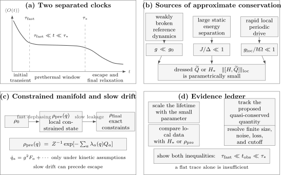
A prethermal claim combines a fast approach, a parametrically later escape, an identified dressed charge or effective Hamiltonian, and a scaling audit. The kinetic form $\dot q_a=g^2F_a+\cdots$ is common but not universal.

What a Plateau Can and Cannot Mean

Observation	Possible interpretation	Missing evidence
local observable becomes nearly constant	dephasing, prethermalization, finite-size saturation, or exact stationarity	a mechanism and an escape scale
approximate charge changes slowly	prethermal constraint	local-state relaxation within its sector
rapid approach to a GGE-like value	near-integrable prethermalization	later drift under integrability breaking
slow energy absorption under a drive	Floquet prethermal protection	equilibration under the effective Hamiltonian
persistent local memory	localization, exact conservation, fragmentation, or a long plateau	transport, perturbation, size, and time scaling
long-lived order	metastability or a prethermal phase	robustness, nucleation or heating mechanism, and lifetime scaling

The word prethermal is justified by a hierarchy, not by nonthermal appearance alone.

Reference Dynamics and Weak Breaking

General setup

Write the exact Hamiltonian as

$$H = H_0 + gV, \qquad |g|\ll g_0,$$

where $H_0$ is a useful reference dynamics. It need not be integrable. Suppose $H_0$ has one or more charges $Q_a$ satisfying

$$[H_0,Q_a]=0,$$

while the perturbation breaks them:

$$[V,Q_a]\neq0.$$

Under the full Hamiltonian,

$$\frac{dQ_a(t)}{dt} = \frac{i g}{\hbar} [V(t),Q_a(t)].$$

This equation identifies the small parameter, but it does not by itself determine the lifetime. The expectation of the commutator may oscillate and average to zero at first order; resonances or coherent secular terms may instead make it accumulate.

A crude norm bound

For a bounded operator,

$$\begin{aligned} \left| \langle Q_a(t)\rangle - \langle Q_a(0)\rangle \right| &\le \frac{|g|}{\hbar} \int_0^t ds \\ &\quad\times \left\| [V(s),Q_a(s)] \right\|. \end{aligned}$$

If the norm is of order one, this only guarantees a time of order $|g|^{-1}$. For extensive operators, the global norm grows with volume and is usually the wrong thermodynamic measure. Local densities, commutators per site, or local interaction norms are the relevant quantities.

Dressed charges

The bare $Q_a$ is often not the longest-lived object. A quasilocal change of basis can construct

$$\widetilde Q_a = e^{-S}Q_a e^S,$$

with

$$\widetilde Q_a = Q_a + gQ_a^{(1)} + g^2Q_a^{(2)} + \cdots.$$

Choosing $S$ order by order can cancel charge-changing terms through some order $n$:

$$[H,\widetilde Q_a^{(n)}] = O\!\left(g^{n+1}\right).$$

The corresponding perturbative estimate is

$$\tau_*^{(n)} \sim \frac{\hbar}{g_0} \left( \frac{g_0}{|g|} \right)^{n+1},$$

up to model-dependent constants and resonances. If the series is asymptotic, there is an optimal order rather than a convergent infinite construction.

Fast equilibration within sectors

Approximate conservation does not itself create a plateau. The reference dynamics must also mix or dephase the chosen probes rapidly while the charges remain nearly fixed.

Let

$$q_a(t) = \frac{1}{L} \langle Q_a(t)\rangle.$$

If $H_0$ equilibrates locally at fixed $q_a$, a moving constrained ensemble can be written

$$\begin{aligned} \rho_{\mathrm{pre}}(q) &= \frac{1}{Z(q)} \exp\!\left[\Xi(q)\right], \\ \Xi(q) &= -\beta(q)H_0 -\sum_a\lambda_a(q)Q_a. \end{aligned}$$

The parameters are chosen to reproduce the instantaneous slowly varying densities. The exact state remains pure if it began pure; the ensemble compresses local information.

Kinetic drift

When first-order secular contributions vanish and the reference dynamics loses memory rapidly enough, second-order perturbation theory often gives

$$\frac{dq_a}{dt} = g^2F_a(q) + O(g^3).$$

The resulting drift time is

$$\tau_* \sim \frac{1}{g^2}$$

in suitable microscopic units. This is the logic behind many quantum Boltzmann equations and the general reference-dynamics framework.

The exponent $2$ is not universal. It can change when:

• a first-order resonance is allowed;
• symmetry forbids the leading transition;
• several particles must cooperate to change the charge;
• the density of final states vanishes or diverges;
• long-time correlations invalidate a Markov approximation;
• the initial state lies near a singular point;
• the perturbation is not small in the relevant local norm.

One should therefore report a measured or derived scaling, not insert $g^{-2}$ by reflex.

Near-Integrable Prethermalization

Approximate charge hierarchy

For

$$H = H_{\mathrm{int}} + gV,$$

an integrable reference Hamiltonian carries charges $Q_r$ with

$$[H_{\mathrm{int}},Q_r]=0.$$

Under the perturbed model,

$$\frac{dQ_r}{dt} = \frac{i g}{\hbar} [V,Q_r].$$

The system can first dephase under $H_{\mathrm{int}}$, producing local values close to a GGE fixed by the initial charge densities. Weak integrability breaking then causes those densities to drift, eventually leaving the GGE manifold or moving along it toward an ordinary thermal state.

The appropriate schematic sequence is

$$\begin{gathered} \rho_0 \\ \Downarrow\quad t\sim\tau_{\mathrm{deph}} \\ \rho_{\mathrm{GGE}}[q_r(0)] \\ \Downarrow\quad t\sim\tau_{\mathrm{break}} \\ \rho_{\mathrm{Gibbs}} \\ \text{or another exact-constraint ensemble}. \end{gathered}$$

Integrability and Generalized Gibbs Ensembles Preview owns the construction and completeness of the GGE. Here the key point is that its charges are only approximate under the full Hamiltonian.

Weakly interacting quasiparticles

A transparent example begins from

$$H_0 = \sum_k \varepsilon_k n_k, \qquad n_k = c_k^\dagger c_k.$$

The mode occupations are exactly conserved by $H_0$. Add a weak two-body interaction $gV$. Coherent dephasing and dressing can occur on a relatively short time, while redistribution of occupations requires collisions.

A schematic fermionic collision integral is

$$\begin{aligned} \dot n_1 &= 2\pi g^2 \sum_{2,3,4} |M_{12;34}|^2 \delta_{\mathbf k} \delta_\varepsilon \mathcal F_{12;34}, \\ \delta_{\mathbf k} &= \delta_{\mathbf k_1+\mathbf k_2,\, \mathbf k_3+\mathbf k_4}, \\ \delta_\varepsilon &= \delta( \varepsilon_1+\varepsilon_2 -\varepsilon_3-\varepsilon_4 ), \\ \mathcal F_{12;34} &= (1-n_1)(1-n_2)n_3n_4 \\ &\quad- n_1n_2(1-n_3)(1-n_4). \end{aligned}$$

The two delta functions impose momentum and energy conservation for the reference quasiparticles. The prefactor displays the common $g^2$ collision scale. On a finite lattice the energy delta function is resolved into discrete levels, so broadening, time windows, and system size must be handled consistently.

Exact integrability is not prethermalization

If $g=0$ exactly and the GGE is stationary forever, the system is integrable rather than prethermal with respect to that charge hierarchy. Prethermalization describes the singular crossover as $g$ becomes small but nonzero.

The order of limits exposes the distinction:

$$\lim_{g\to0} \lim_{t\to\infty} \langle O(t)\rangle \neq \lim_{t\to\infty} \lim_{g\to0} \langle O(t)\rangle$$

whenever the perturbed and integrable endpoints differ.

Large Static Energy Separation

Normal-form structure

Consider a local Hamiltonian

$$H = \Delta N + D + V,$$

where:

$$\begin{gathered} [D,N]=0, \\ \|V\|_{\mathrm{loc}} \sim J, \\ J \ll \Delta. \end{gathered}$$

Assume $N$ has suitably spaced sectors, often an integer spectrum. Terms in $V$ that change $N$ cost the large energy $\Delta$. A quasilocal unitary $Y$ can bring the Hamiltonian to a normal form

$$YHY^\dagger = \Delta N + D_* + E_*,$$

with

$$[D_*,N]=0, \qquad \|E_*\|_{\mathrm{loc}} \ll J.$$

The dressed quantity

$$\widetilde N = Y^\dagger N Y$$

is then almost conserved by the original Hamiltonian. Under theorem-specific locality, boundedness, and spectral assumptions, $E_*$ can be nonperturbatively small and the lifetime nearly exponential or stretched exponential in $\Delta/J$.

It is safer to write the generic message as

$$\tau_* \gg \frac{\hbar}{J}$$

and then state the precise bound for the model at hand.

Large-U Hubbard example

For the Fermi–Hubbard model,

$$H = U N_d + T, \qquad N_d = \sum_i n_{i\uparrow}n_{i\downarrow},$$

where $N_d$ counts doublons and $T$ is hopping. Decompose

$$T = T_{+1} + T_0 + T_{-1},$$

so that

$$[N_d,T_m] = mT_m.$$

For $|U|\gg J$, take the leading anti-Hermitian generator

$$S_1 = \frac{T_{+1}-T_{-1}}{U}.$$

Because

$$[S_1,UN_d] = -T_{+1} -T_{-1},$$

the transformed Hamiltonian has no doublon-changing term at first order:

$$e^{S_1}He^{-S_1} = UN_d + T_0 + O\!\left(\frac{J^2}{U}\right).$$

Thus the bare doublon number is conserved to leading order, while a dressed doublon operator is conserved more accurately. A quench can relax rapidly within a fixed-doublon sector and only later change the doublon density.

This derivation is a scale-separation statement. It does not say that every large-$U$ state is thermal within its sector, nor that doublons never decay.

Gapped low-energy subspaces

Recent rigorous work extends the principle beyond an exactly integer counting operator. For a spatially local gapped Hamiltonian $H_0$ perturbed by local terms of strength $\epsilon\ll\Delta$, local correlation functions can remain close to dynamics restricted to the low-energy subspace for stretched-exponential times under the theorem’s hypotheses.

This result is about local robustness over a long finite time. It is not a blanket claim that the perturbed Hamiltonian remains gapped or that every initial state is protected.

Floquet Prethermalization Preview

Periodic setup

Let

$$H(t+T) = H(t), \qquad \Omega = \frac{2\pi}{T},$$

with one-period propagator

$$U_F = \mathcal T \exp\!\left[ -\frac{i}{\hbar} \int_0^T H(t)\,dt \right].$$

The exact Floquet operator always exists for a well-defined finite problem. The prethermal question is different: can local dynamics for many periods be approximated by a quasilocal static generator?

Local frequency criterion

For an interacting lattice, the global norm $\|H\|$ grows with volume. The thermodynamic control parameter uses a local interaction scale $g_{\mathrm{loc}}$:

$$\eta = \frac{g_{\mathrm{loc}}}{\hbar\Omega}.$$

When $\eta\ll1$ and appropriate locality and bounded-local-Hilbert-space assumptions hold, a periodic dressing $P(t)$ and a quasilocal effective Hamiltonian $H_*$ can approximate

$$U(t) \simeq P(t) \exp\!\left( -\frac{i}{\hbar}H_*t \right) P^\dagger(0)$$

through a long interval. At stroboscopic times, $P(nT)=P(0)$.

Heating suppression

The residual terms that absorb drive quanta are small after optimal truncation. A common schematic estimate is

$$\Gamma_{\mathrm{heat}} \lesssim \frac{g_{\mathrm{loc}}}{\hbar} \exp\!\left[ -c \frac{\hbar\Omega}{g_{\mathrm{loc}}} \right],$$

leading to

$$\tau_* \gtrsim \frac{\hbar}{g_{\mathrm{loc}}} \exp\!\left[ c \frac{\hbar\Omega}{g_{\mathrm{loc}}} \right].$$

Constants, powers, logarithmic corrections, interaction range, smoothness, and precise hypotheses depend on the theorem and model. One rigorous local-spin construction gives a quasi-exponential scale of the form

$$\tau_* \sim \exp\!\left[ c \frac{\Omega} {\log^3(\Omega/\Omega_0)} \right]$$

after nondimensionalizing by a local scale. Other finite-range bounds and physical estimates yield exponential-in-frequency behavior. These statements should not be merged into one universal formula.

High-Frequency Expansions owns the derivations and expansion conventions.

Slow heating is not yet a thermal plateau

There are two logically separate claims:

$$\begin{gathered} \text{heating under the exact drive is slow}, \\ \text{local dynamics under }H_*\text{ equilibrates}. \end{gathered}$$

If $H_*$ is nonintegrable and satisfies ETH in the relevant energy window, a prethermal Gibbs state is plausible:

$$\rho_{\mathrm{pre}} = \frac{ \exp(-\beta_*H_*) }{ \operatorname{Tr}\exp(-\beta_*H_*) }.$$

The inverse temperature $\beta_*$ is fixed approximately by the initial expectation of $H_*$. If $H_*$ is integrable, constrained, fragmented, or localized over the tested window, its local endpoint need not be Gibbs.

Micromotion

Within a drive cycle, observables carry the periodic dressing:

$$O_{\mathrm{lab}}(t) = P(t) O_*P^\dagger(t).$$

A stroboscopic plateau can coexist with substantial intracycle motion. Comparisons must specify whether data are sampled at fixed phase, cycle averaged, or measured continuously.

Prethermalization without temperature

Some driven systems possess an additional approximate symmetry or charge even when the state is effectively at high temperature with respect to $H_*$. Long-lived oscillations or constrained dynamics can then survive without a useful finite prethermal temperature.

This broadens the concept beyond Gibbs plateaus, but the evidence standard remains the same: identify the approximate conserved structure, show its parametric lifetime, and exclude trivial finite-size or calibration effects.

Which Prethermal Ensemble?

Gibbs state of an effective Hamiltonian

If only the effective energy and exact symmetries constrain a locally ergodic $H_*$, use

$$\rho_{\mathrm{pre}} = \frac{1}{Z_*} \exp\!\left( -\beta_*H_* -\sum_\alpha\mu_\alpha C_\alpha \right),$$

where $C_\alpha$ are exact charges.

Generalized prethermal ensemble

If several approximate charges remain fixed over the window,

$$\rho_{\mathrm{pre}} = \frac{1}{Z_{\mathrm{pre}}} \exp\!\left( -\sum_a\lambda_a\widetilde Q_a \right).$$

The charges should be local or quasilocal enough to control the declared probes. Adding arbitrary projectors until a fit succeeds is not a predictive ensemble.

Time-dependent constrained ensemble

When charges drift measurably,

$$\rho_{\mathrm{pre}}(t) = \rho_{\mathrm{pre}}\!\left[q_1(t),q_2(t),\ldots\right].$$

The state can remain close to a moving manifold even though no single stationary density operator fits the entire window.

No ensemble without local relaxation

An effective Hamiltonian can govern dynamics accurately while the initial state continues oscillating or fails to equilibrate under it. In that case, $H_*$ is still useful, but calling $\exp(-\beta_*H_*)/Z_*$ the observed prethermal state would be premature.

Entropy and Information

Exact unitary evolution preserves the global von Neumann entropy:

$$S_{\mathrm{vN}}[\rho(t)] = S_{\mathrm{vN}}[\rho(0)].$$

Prethermal entropy production refers instead to:

• growth of subsystem entanglement entropy;
• dephasing or diagonal entropy in a chosen basis;
• coarse-grained entropy of the prethermal ensemble;
• kinetic entropy associated with slowly evolving occupations.

For a small region $A$,

$$\rho_A(t) = \operatorname{Tr}_{\bar A}\rho(t) \simeq \rho_{A,\mathrm{pre}}$$

can hold while the global state remains far from any mixed ensemble. The plateau entropy may differ from the final thermal entropy because approximate constraints reduce the locally accessible state space.

Timescale and Limit Discipline

A hierarchy ledger

Useful clocks include

Symbol	Meaning
$\tau_{\mathrm{micro}}$	inverse local bandwidth or interaction time
$\tau_{\mathrm{deph}}$	decay of coherent transients under the reference dynamics
$\tau_{\mathrm{loc}}$	local constrained equilibration
$\tau_{\mathrm{tr}}(L)$	transport across system size $L$
$\tau_*$	approximate-charge leakage or drive-heating time
$\tau_{\mathrm{bath}}$	environment-induced relaxation time
$\tau_{\mathrm{rec}}(L)$	finite-size recurrence time

A clean isolated-system prethermal window needs

$$\max( \tau_{\mathrm{deph}}, \tau_{\mathrm{loc}} ) \ll t \ll \min( \tau_*, \tau_{\mathrm{bath}}, \tau_{\mathrm{rec}} ).$$

Transport can be slower than local equilibration, so a spatially inhomogeneous system may require an additional hydrodynamic stage.

Ordered limits

For weak breaking,

$$\lim_{g\to0} \lim_{t\to\infty} \neq \lim_{t\to\infty} \lim_{g\to0}$$

as operations on local observables whenever exact and approximate constraints select different ensembles.

For a driven system,

$$\lim_{\Omega\to\infty} \lim_{t\to\infty} \neq \lim_{t\to\infty} \lim_{\Omega\to\infty}.$$

Taking $\Omega\to\infty$ first can freeze heating; taking $t\to\infty$ first at fixed frequency can reveal eventual absorption.

Finite size

A finite spectrum has a smallest resolved spacing and eventual recurrences. Apparent plateaus can arise when the expected collision width is below that spacing.

For a golden-rule process with rate $\Gamma$ and many-body level spacing $\delta_L$, a continuum kinetic description requires schematically

$$\delta_L \ll \hbar\Gamma \ll g_0.$$

If $\hbar\Gamma\lesssim\delta_L$, increasing time at fixed size does not reproduce the thermodynamic collision integral.

Unbounded local Hilbert spaces

Bosonic lattices and continuum gases do not have a finite maximal local transition energy. A high-frequency or large-gap claim must state:

• the populated energy and occupation window;
• how matrix elements to remote states decay;
• whether losses or three-body processes matter;
• how the Hilbert-space cutoff is varied;
• which resonances remain in the retained window.

An apparent plateau created by truncating away the escape channel is numerical, not physical.

Long-range interactions

Power-law interactions can modify locality bounds and permit collective processes. The relevant norm, system-size dependence, and exponent range must be stated. Short-range exponential-lifetime formulas cannot be transferred unchanged to every dipolar or all-to-all model.

Quantitative Diagnostics

Drift of the proposed charge

For an extensive candidate $\widetilde Q$, define

$$D_Q(t) = \frac{ \left| \langle\widetilde Q(t)\rangle - \langle\widetilde Q(0)\rangle \right| }{ Lq_{\mathrm{ref}} }.$$

The reference scale $q_{\mathrm{ref}}$ should be declared. A prethermal interpretation predicts a parametrically small $D_Q$ over the plateau and a drift correlated with its breakdown.

Effective-dynamics error

For a local observable $O$,

$$\epsilon_O(t) = \left| \langle O(t)\rangle_H - \langle O(t)\rangle_{H_*} \right|.$$

Check $\epsilon_O(t)$ for several support sizes and observables. Agreement for one specially protected operator is weaker than agreement for a local algebra.

Ensemble residual

Given a candidate $\rho_{\mathrm{pre}}$,

$$R_O(t) = \langle O(t)\rangle - \operatorname{Tr} \left( \rho_{\mathrm{pre}}O \right).$$

Report the time average and variance:

$$\overline{R_O} = \frac{1}{t_2-t_1} \int_{t_1}^{t_2} R_O(t)\,dt,$$ $$\sigma_O^2 = \frac{1}{t_2-t_1} \int_{t_1}^{t_2} \left[ R_O(t)-\overline{R_O} \right]^2dt.$$

Small variance with a large bias means the plateau is stable but the proposed ensemble is wrong.

Escape time

Choose a threshold $\epsilon$ before fitting:

$$\tau_*(\epsilon) = \inf \left\{ t>t_1: D_Q(t)\ge\epsilon \right\}.$$

Vary $\epsilon$ to test robustness. A lifetime extracted after inspecting the curve is vulnerable to selection bias.

Parameter scaling

Measure $\tau_*$ as the small parameter is tuned:

$$\tau_*(g) \propto |g|^{-\alpha},$$

or

$$\ln\tau_*(\Omega) \propto \frac{\hbar\Omega}{g_{\mathrm{loc}}},$$

where justified. A fit over less than a decade rarely discriminates a power law from an exponential reliably. Report alternative fits, covariance, and the accessible asymptotic range.

Heating diagnostics

For periodic driving, track the effective energy density

$$e_*(n) = \frac{1}{L} \left\langle H_* \right\rangle_{nT}$$

and a simple infinite-temperature benchmark

$$e_{\infty} = \frac{ \operatorname{Tr}_{\mathcal S}H_* }{ \dim\mathcal S },$$

where $\mathcal S$ is the exact symmetry sector. Energy absorption, entanglement growth, and local-observable relaxation need not share one rate.

Evidence Workflow

1. Specify the protocol. Give $H_0$, the perturbation or drive, the initial state, boundary conditions, and exact symmetry sector.
2. Name the small parameter. Use $|g|/g_0$, $J/\Delta$, or $g_{\mathrm{loc}}/(\hbar\Omega)$ rather than saying only “weak” or “fast.”
3. Identify the reference structure. Construct the bare and, when possible, dressed charge or effective Hamiltonian.
4. Show fast local relaxation. Demonstrate that several probes lose their initial transient while the proposed charge is still fixed.
5. Predict the plateau. Compute local values from $H_*$, a Gibbs state, a GGE, or a moving constrained ensemble.
6. Track slow leakage. Measure the charge drift, heating, or sector-changing transition rate.
7. Scale the lifetime. Vary the perturbation, gap, or frequency and compare with the mechanism-specific prediction.
8. Vary size and cutoffs. Resolve level spacing, recurrences, bond dimension, occupation cutoff, and timestep.
9. Audit the environment. Separate intrinsic leakage from noise, loss, residual coupling, and drive imperfections.
10. State the endpoint and limits. Distinguish an observed lower bound from a demonstrated crossover to the final ensemble.

Representative Experiments

Coherently split one-dimensional Bose gas

Experiments on a coherently split one-dimensional Bose gas observed rapid local emergence of thermal-like phase correlations and a light-cone-like spread of those correlations. The long-lived state retained memory associated with the near-integrable low-energy description. This is a canonical example of local prethermalization without global thermal equilibrium.

The interpretation depends on:

• the Luttinger-liquid or related reference description;
• approximate mode conservation;
• the observable window;
• residual integrability breaking from trapping, transverse modes, and nonlinear corrections.

Long-range interacting spin chains

Trapped-ion experiments observed long-lived quasistationary behavior in spin chains with tunable long-range interactions. Collective constraints and the competition of fluctuation and relaxation times can create a prethermal regime even when the mechanism is not a small perturbation of a conventional short-range integrable model.

Finite system size and interaction range are part of the result. An all-to-all or slowly decaying interaction can have scaling very different from a finite-range lattice theorem.

Floquet Bose–Hubbard systems

Driven optical-lattice experiments measured heating rates in an interacting Bose–Hubbard system and found strong, approximately exponential suppression as the drive frequency increased over the tested regime. The experiment linked the heating curve to the local many-body energy scales and resolved features associated with the equilibrium phase diagram.

The evidence is stronger than a single long-lived trace because frequency, interaction, and dimensionality were varied.

Dipolar spin ensembles

Nuclear-magnetic-resonance experiments in dipolar spin chains observed relaxation to a state described by a prethermal Hamiltonian and exponentially slow heating over an accessible high-frequency range. Tracking the autocorrelation of the effective Hamiltonian directly tested the proposed approximate conservation law.

Additional quasiconserved structures survived after the simplest effective-Hamiltonian picture began to fail, illustrating that several nested prethermal windows can occur.

Experimental error budget

In every platform, compare the intrinsic escape rate with:

$$\begin{aligned} \Gamma_{\mathrm{obs}} &= \Gamma_{\mathrm{intrinsic}} + \Gamma_{\mathrm{noise}} \\ &\quad+ \Gamma_{\mathrm{loss}} + \Gamma_{\mathrm{bath}} \\ &\quad+ \Gamma_{\mathrm{control}}. \end{aligned}$$

Only the sum is measured directly. Frequency scaling, calibration runs, particle-number monitoring, and independent coherence measurements help separate the terms.

Relations to Neighboring Phenomena

Equilibration

A system can equilibrate directly without a parametrically distinct plateau. Prethermalization requires at least two separated relaxation stages.

Exact integrability and GGEs

Exact charges produce stationary constrained behavior. Weakly broken charges can produce a prethermal GGE whose parameters drift. The same density operator can therefore describe an exact endpoint in one Hamiltonian and an intermediate state in a nearby Hamiltonian.

Many-body localization

Idealized MBL retains quasilocal memory asymptotically in an isolated thermodynamic system. A prethermal regime retains memory only over a long finite window. Finite-time data can resemble both, so perturbation, disorder, transport, and lifetime scaling must be compared.

Metastability

Metastability often refers to a particular state or phase protected by an energetic, entropic, or nucleation barrier. Prethermalization usually refers to local relaxation within an almost-invariant sector. The concepts overlap when a metastable sector rapidly develops internal local equilibrium before its rare decay.

Recent rigorous work connects metastable short-range-entangled states to eigenstates of nearby Hamiltonians and bounds local decay for nonperturbatively long times. This enlarges the mathematical setting but does not make every metastable plateau a Gibbs ensemble.

Scars and fragmentation

Quantum scars are atypical states or subspaces with unusual dynamics inside a broader spectrum. Fragmentation splits Hilbert space into disconnected components. Either can generate long-lived signals, but neither is automatically prethermal. A prethermal interpretation needs a tunable approximate constraint and an escape process.

Open-system steady states

A bath can create an attracting stationary state. That is not the same as an isolated prethermal plateau, although weak dissipation can stabilize, destroy, or reshape one. Compare $\tau_{\mathrm{bath}}$ with $\tau_*$ explicitly.

Hydrodynamic plateaus

Slow conserved-density transport can create intermediate spatial profiles. This can coexist with prethermalization, but ordinary diffusion alone does not imply an approximate extra charge.

Common Mistakes

• Calling every shoulder a plateau. Resolve both the approach and escape scales.
• Using one observable. A protected operator can look stationary while the local state drifts.
• Assuming $g^{-2}$ universally. Check first-order resonances, selection rules, and phase space.
• Using a global norm in the thermodynamic limit. State the local interaction scale.
• Equating slow Floquet heating with Gibbs behavior under $H_*$. Internal equilibration is a separate question.
• Dropping micromotion. Stroboscopic and intracycle observables are different.
• Calling an exact GGE prethermal. A finite escape mechanism is part of the latter claim.
• Calling a finite-time MBL-like trace localized. A growing prethermal lifetime can mimic memory.
• Ignoring the bath. Technical heating or loss may set the observed lifetime.
• Fitting an exponential from a narrow frequency range. Compare plausible alternatives and report uncertainty.
• Trusting a Hilbert-space cutoff. Increase it until escape channels and heating rates converge.
• Taking the limits in an unstated order. The plateau can disappear when $t\to\infty$ is taken first.
• Treating $H_*$ as unique. Effective Hamiltonians and dressed observables depend on the chosen frame and truncation convention.
• Inferring a phase from a regime. A prethermal phase needs a dynamical definition and robustness throughout its finite-time window.

Worked Microexamples

Two-rate relaxation model

Let a fast observable $x$ relax toward a value selected by a slow charge $q$:

$$\begin{aligned} \dot x &= -\gamma_f \left[ x-aq \right], \\ \dot q &= -\gamma_s \left[ q-q_{\mathrm{eq}} \right], \end{aligned}$$

with $\gamma_s\ll\gamma_f$. The slow variable is

$$q(t) = q_{\mathrm{eq}} + \left[ q(0)-q_{\mathrm{eq}} \right] e^{-\gamma_st}.$$

After the fast transient,

$$x(t) = aq(t) + O\!\left( \frac{\gamma_s}{\gamma_f} \right).$$

Thus

$$\gamma_f^{-1} \ll t \ll \gamma_s^{-1}$$

gives

$$x(t) \simeq aq(0),$$

while at late times $x(t)\to aq_{\mathrm{eq}}$. The plateau is not perfectly static; its slope is suppressed by $\gamma_s/\gamma_f$.

Why a first-order commutator need not imply a first-order rate

Suppose

$$H = H_0 + gV, \qquad [H_0,Q]=0.$$

In the interaction picture,

$$\begin{aligned} \Delta\langle Q(t)\rangle &= \frac{i g}{\hbar} \int_0^t ds \\ &\quad\times \langle[V_I(s),Q]\rangle_0 + O(g^2). \end{aligned}$$

If the integrand is oscillatory with no zero-frequency component, the integral remains bounded rather than growing linearly. The leading secular drift can then arise at order $g^2t$, giving $\tau_*\sim g^{-2}$. If a resonance supplies a zero-frequency component, the order-$g$ term can grow and the lifetime is shorter.

Floquet energy and local-state clocks

Suppose a drive has heating rate

$$\Gamma_{\mathrm{heat}} \sim \frac{g_{\mathrm{loc}}}{\hbar} e^{-c\hbar\Omega/g_{\mathrm{loc}}},$$

while $H_*$ locally equilibrates at rate $\Gamma_{\mathrm{loc}}\sim g_{\mathrm{loc}}/\hbar$. Then

$$\frac{\tau_*}{\tau_{\mathrm{loc}}} \sim e^{c\hbar\Omega/g_{\mathrm{loc}}}.$$

The exponential controls the ratio of clocks, not the absolute quality of a low-order expansion. One still checks resonances, micromotion, and the first omitted term.

Exercises

1. Order of limits

Consider

$$O_g(t) = O_{\mathrm{th}} + \left( O_{\mathrm{pre}}-O_{\mathrm{th}} \right) e^{-g^2t}.$$

Evaluate the two ordered limits $g\to0$ and $t\to\infty$. Interpret the result.

Solution

At fixed $g\neq0$,

$$\lim_{t\to\infty} O_g(t) = O_{\mathrm{th}},$$

so

$$\lim_{g\to0} \lim_{t\to\infty} O_g(t) = O_{\mathrm{th}}.$$

At fixed $t$,

$$\lim_{g\to0} O_g(t) = O_{\mathrm{pre}},$$

and therefore

$$\lim_{t\to\infty} \lim_{g\to0} O_g(t) = O_{\mathrm{pre}}.$$

The exact integrable point has an indefinitely stable constrained value, whereas every fixed nonzero breaking eventually reaches the thermal value. The prethermal plateau occupies the singular intermediate window $1\ll t\ll g^{-2}$.

2. Crude approximate-charge bound

Let $[H_0,Q]=0$, $H=H_0+gV$, and $\|[V,Q]\|\le C$. Show that

$$\left| \langle Q(t)\rangle-\langle Q(0)\rangle \right| \le \frac{|g|Ct}{\hbar}.$$

What does this prove, and what does it fail to prove?

Solution

The Heisenberg equation gives

$$\frac{d}{dt} \langle Q(t)\rangle = \frac{i g}{\hbar} \langle[V(t),Q(t)]\rangle.$$

Using $|\langle A\rangle|\le\|A\|$ and unitary invariance of the norm,

$$\left| \frac{d}{dt} \langle Q(t)\rangle \right| \le \frac{|g|C}{\hbar}.$$

Integration yields the stated inequality. It guarantees small drift only up to a scale of order $|g|^{-1}$ for fixed tolerance. It does not prove that this scale is sharp, that the system locally equilibrates, or that cancellations cannot extend the lifetime to $g^{-2}$ or a nonperturbative scale. For extensive $Q$, one also needs a local or density-normalized version.

3. Maximum-entropy prethermal state

Suppose the effective dynamics conserves $H_*$ and an approximate charge $\widetilde Q$ over the observation window. Maximize

$$S = -\operatorname{Tr}(\rho\ln\rho)$$

subject to normalization and fixed expectations of $H_*$ and $\widetilde Q$.

Solution

Introduce multipliers $\alpha$, $\beta_*$, and $\lambda$ and vary

$$\begin{aligned} \mathcal L &= S -\alpha( \operatorname{Tr}\rho-1 ) \\ &\quad- \beta_* \left( \operatorname{Tr}\rho H_*-E_* \right) \\ &\quad- \lambda \left( \operatorname{Tr}\rho\widetilde Q-q_* \right). \end{aligned}$$

Stationarity gives

$$\ln\rho = -1-\alpha-\beta_*H_*-\lambda\widetilde Q,$$

so

$$\rho_{\mathrm{pre}} = \frac{1}{Z} \exp\!\left( -\beta_*H_*-\lambda\widetilde Q \right).$$

This is predictive only if the chosen charges are physically justified and the dynamics equilibrates locally within their sectors.

4. Solve the two-rate model

For

$$\dot x = -\gamma_f(x-aq), \qquad \dot q = -\gamma_s(q-q_{\mathrm{eq}}),$$

derive the exact $x(t)$ for $\gamma_f\neq\gamma_s$.

Solution

First,

$$\begin{aligned} q(t) &= q_{\mathrm{eq}} + \Delta q\,e^{-\gamma_st}, \\ \Delta q &= q(0)-q_{\mathrm{eq}}. \end{aligned}$$

Using an integrating factor for $x$,

$$\begin{aligned} x(t) &= aq_{\mathrm{eq}} + \left[ x(0)-aq_{\mathrm{eq}} \right] e^{-\gamma_ft} \\ &\quad+ \frac{a\gamma_f\Delta q} {\gamma_f-\gamma_s} \left( e^{-\gamma_st} - e^{-\gamma_ft} \right). \end{aligned}$$

For $\gamma_s\ll\gamma_f$ and $\gamma_f^{-1}\ll t\ll\gamma_s^{-1}$,

$$x(t) \simeq aq(0) + O\!\left( \frac{\gamma_s}{\gamma_f} \right).$$

5. Selection-rule scaling

Suppose changing an approximate charge requires $k$ applications of a perturbation $gV$. Estimate the leading transition amplitude and golden-rule rate.

Solution

If all lower orders vanish by a selection rule, the first nonzero effective matrix element is schematically

$$M_{\mathrm{eff}} \sim g^k \prod_{j=1}^{k-1} \frac{1}{\Delta_j},$$

where $\Delta_j$ are intermediate-state detunings. A golden-rule rate is quadratic in the matrix element:

$$\Gamma \sim \frac{2\pi}{\hbar} |M_{\mathrm{eff}}|^2 \rho_f.$$

If the detunings remain of microscopic order and the final density of states $\rho_f$ is nonsingular,

$$\Gamma \propto g^{2k}, \qquad \tau_* \propto g^{-2k}.$$

Resonant denominators, vanishing phase space, or coherent dynamics can invalidate this estimate.

6. Leading Hubbard transformation

Verify that

$$S_1 = \frac{T_{+1}-T_{-1}}{U}$$

cancels $T_{+1}+T_{-1}$ to first order in $e^{S_1}He^{-S_1}$.

Solution

Use

$$[N_d,T_m] = mT_m.$$

Therefore

$$[T_{+1},N_d] = -T_{+1}, \qquad [T_{-1},N_d] = T_{-1}.$$

It follows that

$$[S_1,UN_d] = -T_{+1} -T_{-1}.$$

The Baker–Campbell–Hausdorff expansion begins

$$e^{S_1}He^{-S_1} = H+[S_1,H]+\cdots.$$

Hence the commutator with $UN_d$ cancels the charge-changing hopping at order $J$, leaving $UN_d+T_0$ plus terms of order $J^2/U$.

7. Stroboscopic versus intracycle plateaus

Suppose

$$\begin{aligned} U(t) &\simeq P(t)e^{-iH_*t/\hbar}P^\dagger(0), \\ P(t+T) &= P(t). \end{aligned}$$

Show how the expectation of a laboratory observable differs from that of its dressed representative.

Solution

For an initial state $\rho_0$,

$$\langle O\rangle_t = \operatorname{Tr} \left[ \rho_0 U^\dagger(t)OU(t) \right].$$

Substituting the factorization gives evolution under $H_*$ of

$$O_*(t) = P^\dagger(t)OP(t),$$

with the initial state dressed by $P^\dagger(0)$. At $t=nT$, periodicity gives $P(nT)=P(0)$, so the same dressed observable is sampled each cycle. At intermediate phases, $P(t)$ changes and can produce substantial micromotion even when the stroboscopic sequence is flat.

8. Design a decisive test

A local magnetization remains nearly constant for all measured times as a weak perturbation $g$ is varied. List a minimal set of additional measurements needed to distinguish prethermalization from exact conservation, finite-size freezing, localization, and technical decoherence.

Solution

A useful test set is:

1. compute or measure the commutator of the proposed bare or dressed charge with the full Hamiltonian;
2. measure several local observables and correlations, not only the magnetization;
3. vary $g$ over a range sufficient to test a lifetime law;
4. increase size so that level spacing and recurrence effects change;
5. measure transport or spatial spreading to test localization;
6. perturb disorder and integrability independently;
7. monitor particle loss, control noise, and bath coherence times;
8. extend the window until drift appears or report only a lower bound on $\tau_*$;
9. compare the plateau values with a predicted $H_*$, Gibbs state, or GGE;
10. state the order of thermodynamic, long-time, and weak-coupling limits.

Together these measurements test the mechanism, local-state prediction, scaling, alternatives, and endpoint.

Status Ledger

Claim	Status
separated fast and slow processes can produce long-lived intermediate local regimes	established across many models and platforms
weakly broken reference charges can generate slow motion on a constrained-equilibrium manifold	established under kinetic and mixing assumptions; details are model dependent
$g^{-2}$ is a common weak-breaking lifetime	common, not universal
local high-frequency drives admit long-lived effective Hamiltonians	rigorous under specific locality, boundedness, and frequency hypotheses
high-frequency Floquet heating is always absent	false; generic systems can heat at sufficiently late times
every prethermal plateau has a temperature	false
large static gaps protect local subspaces for nonperturbatively long times	rigorous for important classes; precise bounds require the theorem’s hypotheses
long-range, unbounded, aperiodic, and metastable settings follow one universal lifetime law	active and model dependent

The core concept is standard. The rapidly developing frontier concerns how far rigorous locality methods extend, which engineered drives produce hierarchical constraints, how metastability and scars fit into the same normal-form language, and how prethermal phases survive in realistic noisy devices.

References

1. J. Berges, S. Borsányi, and C. Wetterich, “Prethermalization,” Physical Review Letters 93, 142002 (2004). doi:10.1103/PhysRevLett.93.142002
2. M. Moeckel and S. Kehrein, “Interaction quench in the Hubbard model,” Physical Review Letters 100, 175702 (2008). doi:10.1103/PhysRevLett.100.175702
3. M. Kollar, F. A. Wolf, and M. Eckstein, “Generalized Gibbs ensemble prediction of prethermalization plateaus and their relation to nonthermal steady states in integrable systems,” Physical Review B 84, 054304 (2011). doi:10.1103/PhysRevB.84.054304
4. M. Gring et al., “Relaxation and prethermalization in an isolated quantum system,” Science 337, 1318–1322 (2012). doi:10.1126/science.1224953
5. T. Langen, R. Geiger, M. Kuhnert, B. Rauer, and J. Schmiedmayer, “Local emergence of thermal correlations in an isolated quantum many-body system,” Nature Physics 9, 640–643 (2013). doi:10.1038/nphys2739
6. M. Marcuzzi, J. Marino, A. Gambassi, and A. Silva, “Prethermalization in a nonintegrable quantum spin chain after a quench,” Physical Review Letters 111, 197203 (2013). doi:10.1103/PhysRevLett.111.197203
7. B. Bertini, F. H. L. Essler, S. Groha, and N. J. Robinson, “Prethermalization and thermalization in models with weak integrability breaking,” Physical Review Letters 115, 180601 (2015). doi:10.1103/PhysRevLett.115.180601
8. T. Mori, T. N. Ikeda, E. Kaminishi, and M. Ueda, “Thermalization and prethermalization in isolated quantum systems: a theoretical overview,” Journal of Physics B 51, 112001 (2018). doi:10.1088/1361-6455/aabcdf
9. K. Mallayya, M. Rigol, and W. De Roeck, “Prethermalization and thermalization in isolated quantum systems,” Physical Review X 9, 021027 (2019). doi:10.1103/PhysRevX.9.021027
10. D. Abanin, W. De Roeck, W. W. Ho, and F. Huveneers, “A rigorous theory of many-body prethermalization for periodically driven and closed quantum systems,” Communications in Mathematical Physics 354, 809–827 (2017). doi:10.1007/s00220-017-2930-x
11. T. Mori, T. Kuwahara, and K. Saito, “Rigorous bound on energy absorption and generic relaxation in periodically driven quantum systems,” Physical Review Letters 116, 120401 (2016). doi:10.1103/PhysRevLett.116.120401
12. T. Kuwahara, T. Mori, and K. Saito, “Floquet–Magnus theory and generic transient dynamics in periodically driven many-body quantum systems,” Annals of Physics 367, 96–124 (2016). doi:10.1016/j.aop.2016.01.012
13. D. A. Abanin, W. De Roeck, W. W. Ho, and F. Huveneers, “Effective Hamiltonians, prethermalization, and slow energy absorption in periodically driven many-body systems,” Physical Review B 95, 014112 (2017). doi:10.1103/PhysRevB.95.014112
14. D. V. Else, B. Bauer, and C. Nayak, “Prethermal phases of matter protected by time-translation symmetry,” Physical Review X 7, 011026 (2017). doi:10.1103/PhysRevX.7.011026
15. A. Rubio-Abadal et al., “Floquet prethermalization in a Bose–Hubbard system,” Physical Review X 10, 021044 (2020). doi:10.1103/PhysRevX.10.021044
16. D. J. Luitz, R. Moessner, S. L. Sondhi, and V. Khemani, “Prethermalization without temperature,” Physical Review X 10, 021046 (2020). doi:10.1103/PhysRevX.10.021046
17. P. Peng, C. Yin, X. Huang, C. Ramanathan, and P. Cappellaro, “Floquet prethermalization in dipolar spin chains,” Nature Physics 17, 444–447 (2021). doi:10.1038/s41567-020-01120-z
18. B. Neyenhuis et al., “Observation of prethermalization in long-range interacting spin chains,” Science Advances 3, e1700672 (2017). doi:10.1126/sciadv.1700672
19. W. W. Ho, I. Protopopov, and D. A. Abanin, “Bounds on energy absorption and prethermalization in quantum systems with long-range interactions,” Physical Review Letters 120, 200601 (2018). doi:10.1103/PhysRevLett.120.200601
20. F. Machado, G. D. Kahanamoku-Meyer, D. V. Else, C. Nayak, and N. Y. Yao, “Long-range prethermal phases of nonequilibrium matter,” Physical Review X 10, 011043 (2020). doi:10.1103/PhysRevX.10.011043
21. D. V. Else, W. W. Ho, and P. T. Dumitrescu, “Long-lived interacting phases of matter protected by multiple time-translation symmetries in quasiperiodically driven systems,” Physical Review X 10, 021032 (2020). doi:10.1103/PhysRevX.10.021032
22. C. Fleckenstein and M. Bukov, “Prethermalization and thermalization in periodically driven many-body systems away from the high-frequency limit,” Physical Review B 103, L140302 (2021). doi:10.1103/PhysRevB.103.L140302
23. C. Yin and A. Lucas, “Prethermalization and the local robustness of gapped systems,” Physical Review Letters 131, 050402 (2023). doi:10.1103/PhysRevLett.131.050402
24. N. O’Dea, F. Burnell, A. Chandran, and V. Khemani, “Prethermal stability of eigenstates under high-frequency Floquet driving,” Physical Review Letters 132, 100401 (2024). doi:10.1103/PhysRevLett.132.100401
25. C. Yin, F. M. Surace, and A. Lucas, “Theory of metastable states in many-body quantum systems,” Physical Review X 15, 011064 (2025). doi:10.1103/PhysRevX.15.011064
26. T. Langen, T. Gasenzer, and J. Schmiedmayer, “Prethermalization and universal dynamics in near-integrable quantum systems,” Journal of Statistical Mechanics 2016, 064009 (2016). doi:10.1088/1742-5468/2016/06/064009
27. A. Mitra, “Correlation functions in the prethermalized regime after a quantum quench of a spin chain,” Physical Review B 87, 205109 (2013). doi:10.1103/PhysRevB.87.205109

Summary

• Prethermalization is a hierarchy $\tau_{\mathrm{fast}}\ll t\ll\tau_*$, not merely a flat trace.
• Approximate charges or an effective Hamiltonian organize fast local relaxation while weak leakage controls the later drift.
• Near-integrable kinetic lifetimes, static large-gap lifetimes, and Floquet heating times obey different assumptions and need not share one scaling law.
• A prethermal state may be Gibbs, generalized, time dependent, or not meaningfully thermal at all.
• Strong evidence combines local-state prediction, charge drift, lifetime scaling, finite-size and cutoff control, environmental calibration, and an explicit endpoint.