Floquet Systems Preview

A Floquet many-body system is an interacting quantum system driven by a Hamiltonian that repeats after a period $T$. Its exact one-cycle propagator is a unitary Floquet operator, but the many-body consequences are not exhausted by diagonalizing that operator. The quasienergy zone has fixed width $\hbar\Omega$, while the number of states in a symmetry sector usually grows exponentially with system size. Resonances therefore become dense, generic isolated systems can absorb energy until local observables approach a sector-constrained infinite-temperature state, and a useful local effective Hamiltonian exists only in controlled regimes.

Periodic driving nevertheless creates valuable windows of dynamics. At high local drive frequency, heating can be exponentially slow and a quasilocal effective Hamiltonian can govern a long prethermal interval. Carefully designed cycles can renormalize tunneling, synthesize gauge fields, modify exchange, pump quantum information, or support robust subharmonic response. Baths can instead stabilize a periodic nonequilibrium steady state. Each claim requires its own lifetime, scaling, and error ledger.

Purpose and Canonical Scope

This page is the many-body regime map for periodic quantum driving. It owns:

• the exponential spectral crowding that distinguishes many-body Floquet systems from few-level examples;
• Floquet eigenstate thermalization and sector-constrained heating;
• the competition among generic heating, high-frequency prethermalization, localization or constraints, and dissipation;
• many-body Floquet engineering;
• previews of discrete time crystals and anomalous Floquet phases;
• numerical and experimental standards for deciding which regime has actually been observed.

Several neighboring pages own the underlying machinery:

• Floquet Theorem in Quantum Mechanics proves the exact theorem and introduces periodic modes.
• Floquet Operators owns reference-phase dependence, logarithm branches, and exact stroboscopic propagation.
• Quasienergies owns Floquet zones, gauge equivalence, and extended Floquet space.
• High-Frequency Expansions owns van Vleck expansions, kick operators, and truncation control.
• Floquet–Magnus Expansion owns the phase-dependent one-cycle Magnus construction.
• Driven Many-Body Systems owns exact power ledgers, absorption measures, loss controls, and driven–dissipative energy balance.
• Prethermalization Preview owns the general definition and evidence standards for a prethermal plateau.

The word preview matters. Exact Floquet kinematics is standard. Heating bounds are rigorous under specified locality and boundedness assumptions. The stability and classification of interacting Floquet phases depend more strongly on dimensionality, disorder, interaction range, environment, and the order of limits.

Periodic Many-Body Setup

Let

$$H(t+T)=H(t), \qquad \Omega=\frac{2\pi}{T}.$$

For a lattice system, locality is expressed schematically as

$$H(t) = \sum_{X\subset\Lambda} h_X(t),$$

where $h_X(t)$ acts on a finite region $X$ or decays sufficiently rapidly with its diameter. A local energy scale may be defined, for example, by

$$J \sim \sup_t \max_{i\in\Lambda} \sum_{X\ni i} \lVert h_X(t)\rVert.$$

The precise norm entering a theorem depends on the locality assumptions. The important comparison is usually $\hbar\Omega/J$, not $\hbar\Omega/\lVert H\rVert$. For an extensive Hamiltonian, $\lVert H\rVert$ normally grows with system size even when the local scale $J$ remains fixed.

Choose a reference phase $t_0$. The one-period propagator is

$$\begin{aligned} U_F(t_0) &\equiv U(t_0+T,t_0) \\ &= \mathcal T \exp \left[ -\frac{i}{\hbar} \int_{t_0}^{t_0+T} H(s)\,ds \right]. \end{aligned}$$

At stroboscopic times,

$$U(t_0+nT,t_0) = U_F(t_0)^n.$$

For a two-step drive,

$$H(t) = \begin{cases} H_1, & 0\le t<T_1, \\ H_2, & T_1\le t<T, \end{cases}$$

with $T=T_1+T_2$, one obtains

$$U_F = e^{-iH_2T_2/\hbar} e^{-iH_1T_1/\hbar}.$$

The order is physical. Reversing the factors describes a different protocol unless the two generators commute or the change is exactly a shift of the cycle origin.

Eigenphases and quasienergies

In a finite Hilbert space, write

$$U_F(t_0) \lvert\phi_\alpha(t_0)\rangle = e^{-i\theta_\alpha} \lvert\phi_\alpha(t_0)\rangle.$$

One may define

$$\varepsilon_\alpha = \frac{\hbar\theta_\alpha}{T},$$

but

$$\varepsilon_\alpha \sim \varepsilon_\alpha + m\hbar\Omega, \qquad m\in\mathbb Z.$$

The eigenvalue $e^{-i\theta_\alpha}$ is invariant under this relabeling. A chosen quasienergy is not.

Changing $t_0$ conjugates the Floquet operator:

$$\begin{aligned} U_F(t_1) &= U(t_1,t_0) U_F(t_0) U(t_1,t_0)^\dagger. \end{aligned}$$

Its eigenphases are therefore independent of the cycle origin, while eigenvectors and intracycle observables transform with micromotion.

Why the Many-Body Limit Is Different

Consider a symmetry sector $q$ of dimension $\mathcal D_q$. For a finite-density lattice system,

$$\mathcal D_q \sim e^{s_q N}$$

up to subexponential factors, where $N$ is the number of sites and $s_q$ is an entropy density. All eigenphases fit on a circle of circumference $2\pi$. A typical mean phase spacing therefore scales as

$$\delta\theta_q \sim \frac{2\pi}{\mathcal D_q},$$

and the corresponding quasienergy spacing is

$$\delta\varepsilon_q \sim \frac{\hbar\Omega}{\mathcal D_q} \sim \hbar\Omega e^{-s_qN}.$$

This exponential crowding is the basic many-body obstruction. A frequency can be much larger than every local matrix element while still being far smaller than the full many-body bandwidth. As $N$ grows, folded levels encounter exponentially many near-degeneracies. Generic perturbations turn many of them into avoided crossings.

No quasienergy ground state

Quasienergy lives on a circle. There is no invariant lowest quasienergy and no general principle that fills a Floquet spectrum from the bottom. Phrases such as Floquet ground state are meaningful only after specifying an effective Hamiltonian, a branch, a preparation protocol, and a time window in which that description is controlled.

The formal logarithm

$$H_F(t_0) = \frac{i\hbar}{T} \log U_F(t_0)$$

always exists for a finite-dimensional unitary after choosing branches. It need not be local, smoothly connected as parameters vary, or thermodynamically useful. The existence of a matrix logarithm is therefore much weaker than the existence of a quasilocal effective Hamiltonian.

Adiabatic following is fragile

For a few isolated levels, a slowly ramped periodic drive may follow a chosen quasienergy branch. In a many-body system, the minimum avoided-crossing gap generally shrinks rapidly with size. A ramp slow enough to be globally adiabatic can then traverse unwanted resonances, while a faster ramp creates excitations relative to the desired effective Hamiltonian.

A practical preparation window often has the form

$$\tau_{\mathrm{local}} \ll \tau_{\mathrm{ramp}} \ll t_*,$$

where $\tau_{\mathrm{local}}$ is a local adjustment time and $t_*$ is the heating or escape time. This is a finite-time control criterion, not a global quasienergy adiabatic theorem.

Floquet Dephasing and the Diagonal Ensemble

Expand an initial pure state in a nondegenerate Floquet basis:

$$\lvert\psi_0\rangle = \sum_\alpha c_\alpha \lvert\phi_\alpha\rangle.$$

After $n$ cycles,

$$\lvert\psi_n\rangle = \sum_\alpha c_\alpha e^{-in\theta_\alpha} \lvert\phi_\alpha\rangle.$$

For an observable $O$ sampled at the same drive phase,

$$\begin{aligned} \langle O\rangle_n &= \sum_{\alpha,\beta} c_\alpha^*c_\beta e^{in(\theta_\alpha-\theta_\beta)} O_{\alpha\beta}. \end{aligned}$$

If nondegenerate phase differences dephase under a long-time average, then

$$\overline{\langle O\rangle} = \sum_\alpha \lvert c_\alpha\rvert^2 O_{\alpha\alpha}.$$

Equivalently,

$$\rho_{\mathrm{diag}}^{F} = \sum_\alpha \lvert c_\alpha\rvert^2 \lvert\phi_\alpha\rangle \langle\phi_\alpha\rvert.$$

Exact quasienergy degeneracies require projectors onto degenerate eigenspaces:

$$\rho_{\mathrm{diag}}^{F} = \sum_\lambda P_\lambda\rho_0P_\lambda.$$

The diagonal ensemble explains loss of phase coherence between Floquet eigenstates. It does not by itself establish thermalization. Thermal behavior requires information about the diagonal matrix elements $O_{\alpha\alpha}$.

Floquet Eigenstate Thermalization

For a generic interacting, isolated, chaotic Floquet system with a finite local Hilbert space, Floquet eigenstates are expected to look locally like infinite-temperature states within each exact symmetry sector. If $P_q$ projects onto sector $q$ and

$$\mathcal D_q = \operatorname{Tr}P_q,$$

the sector identity state is

$$\rho_{\infty,q} = \frac{P_q}{\mathcal D_q}.$$

Floquet eigenstate thermalization predicts, for suitable few-body observables,

$$\langle\phi_\alpha|O|\phi_\alpha\rangle \approx \operatorname{Tr} \left( \rho_{\infty,q}O \right)$$

for eigenstates in sector $q$, with finite-size fluctuations that decrease as the sector grows. If the initial state has weights

$$p_q = \operatorname{Tr}(P_q\rho_0),$$

the late local state is expected to approach

$$\rho_\infty^{\mathrm{acc}} = \sum_q p_q \frac{P_q}{\mathcal D_q}.$$

This is not always the full identity divided by the total Hilbert-space dimension. Particle number, parity, lattice momentum, gauge constraints, or other exact symmetries restrict what is dynamically accessible.

Infinite temperature is an observable statement

Unitary evolution preserves the von Neumann entropy of the entire closed system. Heating to infinite temperature means that local observables, reduced states, and sufficiently coarse probes approach the predictions of $\rho_\infty^{\mathrm{acc}}$. Entanglement and diagonal entropy can grow even though the global state remains pure.

With a reference Hamiltonian $H_{\mathrm{ref}}$, define

$$e_{\mathrm{ref}}(n) = \frac{1}{N} \operatorname{Tr} \left[ \rho(nT)H_{\mathrm{ref}} \right].$$

The symmetry-constrained infinite-temperature benchmark is

$$e_{\infty}^{\mathrm{acc}} = \frac{1}{N} \operatorname{Tr} \left[ \rho_\infty^{\mathrm{acc}} H_{\mathrm{ref}} \right].$$

Approach of one energy proxy to this number is useful but not conclusive. A heating claim should also examine local observables, entanglement or entropy proxies, conserved-sector weights, and loss.

Unbounded local Hilbert spaces

Bosonic and continuum systems need extra care. The identity is not trace class on an infinite-dimensional local Hilbert space, so a literal normalized infinite-temperature state may not exist. Occupation cutoffs, trap loss, multiparticle bands, and ultraviolet physics can determine what is observed. The correct conclusion may be continued energy growth or escape from the retained model rather than convergence to a maximally mixed state.

Spectral Diagnostics on the Unit Circle

Order the eigenphases in a fixed symmetry sector:

$$0\le \theta_1 \le\cdots\le \theta_{\mathcal D_q} <2\pi.$$

Define circular gaps

$$s_\alpha = \theta_{\alpha+1} -\theta_\alpha,$$

with

$$s_{\mathcal D_q} = 2\pi +\theta_1 -\theta_{\mathcal D_q}.$$

A branch-independent adjacent-gap ratio is

$$r_\alpha = \frac{ \min(s_\alpha,s_{\alpha+1}) }{ \max(s_\alpha,s_{\alpha+1}) }.$$

Chaotic Floquet operators commonly show circular-ensemble level repulsion, with the relevant ensemble fixed by antiunitary and other symmetries. Integrable or localized models often show nearly Poisson phase statistics. This diagnostic is meaningful only after resolving every exact symmetry and removing accidental block structure.

Level statistics are not a complete phase diagnosis. Small systems can look random before local observables heat, while a mixture of unresolved sectors can look Poisson even when each block is chaotic.

Four Routes Through a Floquet Problem

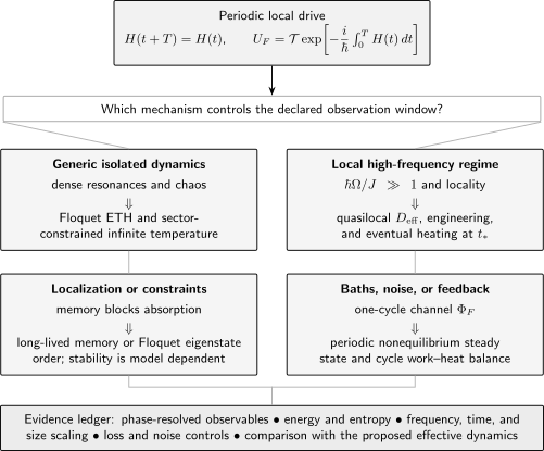
The same exact Floquet operator can sit in very different physical regimes. A regime claim needs dynamical evidence: spectral structure alone does not establish heating, prethermal control, eigenstate order, or a bath-stabilized limit cycle.

The four branches are not exhaustive, and their boundaries can cross:

Regime	Stabilizing or destabilizing mechanism	Typical late or intermediate behavior	Main caveat
Generic isolated ergodic	Dense resonances and operator mixing	Sector-constrained Floquet-ETH behavior	Heating time may exceed the observation window
High-frequency prethermal	Locality and $\hbar\Omega/J\gg1$	Effective-Hamiltonian dynamics for $t\ll t_*$	Eventual heating remains possible
Localized or constrained	Disorder, integrability, fragmentation, or selection rules	Memory and possible Floquet eigenstate order	Stability can fail under perturbations or in larger systems
Open periodically driven	Dissipation competes with work input	Periodic nonequilibrium steady state	The state is generally not Gibbs and depends on bath modeling

The relevant question is not simply “What is $H_F$?” It is:

Over which observables, length scales, drive phases, system sizes, and times does a proposed effective description predict the measured dynamics?

High-Frequency Floquet Prethermalization

For a local drive with

$$\frac{\hbar\Omega}{J} \gg 1,$$

one can often construct a quasilocal effective generator $D_{\mathrm{eff}}$ and a periodic kick or micromotion operator $K(t)$. Over a long but finite interval,

$$\begin{aligned} U(t_0+nT,t_0) &\approx e^{-iK(t_0)} \\ &\quad\times e^{-iD_{\mathrm{eff}}nT/\hbar} e^{iK(t_0)}. \end{aligned}$$

The approximation is local: it controls few-body observables and energy absorption under stated assumptions. It should not be read as a uniform small error in the full many-body operator norm at arbitrarily large $N$.

For broad classes of short-range, bounded local systems, the heating time has an exponential form up to model-dependent constants,

$$t_* \gtrsim \tau_0 \exp \left( c\frac{\hbar\Omega}{J} \right).$$

Equivalently, a heating rate can be exponentially small,

$$\Gamma_{\mathrm{heat}} \lesssim \Gamma_0 \exp \left( -c\frac{\hbar\Omega}{J} \right).$$

Neither expression is universal without its assumptions. Constants depend on locality, interaction range, waveform, and norm convention. Bosonic systems with unbounded onsite occupation need occupancy or energy-window control.

Effective conservation

Within the prethermal interval, the dressed operator

$$\widetilde D = e^{-iK(t_0)} D_{\mathrm{eff}} e^{iK(t_0)}$$

changes slowly under repeated cycles. A useful audit measures

$$\delta_D(n) = \frac{1}{N} \left| \langle\widetilde D\rangle_n -\langle\widetilde D\rangle_0 \right|.$$

Small $\delta_D(n)$ is evidence for approximate conservation. It is not enough by itself to show that the system has relaxed to a Gibbs state of $D_{\mathrm{eff}}$. One must separately test local equilibration and ensemble predictions.

The truncation is asymptotic

An inverse-frequency expansion has terms schematically of size

$$D_{\mathrm{eff}}^{(m)} \sim J \left( \frac{J}{\hbar\Omega} \right)^m m!,$$

where the factorial is a schematic reminder of proliferating nested commutators. The best approximation is commonly obtained by truncating near an optimal order

$$m_* \sim \frac{\hbar\Omega}{J},$$

not by summing indefinitely. High-Frequency Expansions gives the controlled constructions and convention dependence.

Resonances set the boundary

If a local transition of energy $\Delta$ satisfies

$$\Delta \approx m\hbar\Omega,$$

an $m$-quantum process can become resonant. A resonance may be useful when intentionally isolated, but a dense network of resonances destroys a simple off-resonant expansion. Near resonance, the relevant states should be retained in a rotating-frame or degenerate effective theory rather than hidden in a small denominator.

Prethermal does not mean static

Micromotion remains present:

$$K(t+T)=K(t).$$

Two observables measured at different phases of a cycle can differ even if their stroboscopic envelopes follow the same $D_{\mathrm{eff}}$. A high-frequency experiment should therefore record the phase of every measurement and, when feasible, resolve at least one full cycle.

Floquet Engineering

Floquet engineering uses periodic driving to create a controlled effective generator or a controlled unitary cycle. It is successful only when the engineered effect is larger than heating, leakage, decoherence, calibration uncertainty, and neglected higher-order terms over the intended observation time.

Shaken-lattice tunneling

Consider nearest-neighbor hopping with a periodic Peierls phase,

$$H_J(t) = -J \sum_j \left[ e^{i\kappa\sin(\Omega t)} a_{j+1}^\dagger a_j + \text{h.c.} \right].$$

The Jacobi–Anger expansion gives

$$e^{i\kappa\sin(\Omega t)} = \sum_{m\in\mathbb Z} \mathcal J_m(\kappa) e^{im\Omega t},$$

where $\mathcal J_m$ is a Bessel function. Period averaging yields the leading hopping

$$J_{\mathrm{eff}} = J\mathcal J_0(\kappa).$$

At a zero of $\mathcal J_0$, the leading nearest-neighbor hopping vanishes. This is not an exact statement about the full driven many-body system. Higher-order tunneling, interactions, micromotion, band excitation, and heating remain.

Interaction-dressed exchange

In a driven Hubbard regime, virtual doublon–holon processes can absorb or emit drive quanta. A schematic exchange scale is

$$J_{\mathrm{ex}}^{F} \approx 4J^2 \sum_{m\in\mathbb Z} \frac{ \mathcal J_m(\kappa)^2 }{ U+m\hbar\Omega }.$$

This formula displays the main physics: the drive redistributes virtual processes among photon sectors and can modify both magnitude and sign. It ceases to be a harmless off-resonant expression when a denominator approaches zero. Then real doublon production, finite ramp speed, and higher bands must be included.

Synthetic gauge structure

Circular or spatially patterned modulation can generate complex hopping amplitudes,

$$J_{ij}^{\mathrm{eff}} = \lvert J_{ij}^{\mathrm{eff}}\rvert e^{iA_{ij}},$$

with a plaquette phase

$$\Phi_{\mathcal P} = \sum_{\langle ij\rangle\in\mathcal P} A_{ij}.$$

The resulting effective Hamiltonian can imitate a magnetic flux or a topological band model. The Haldane-model realization in a shaken honeycomb lattice is a canonical example. A complete claim requires more than a fitted $H_{\mathrm{eff}}$: it should compare measured gaps, transport or Berry-curvature proxies, micromotion, loading fidelity, and heating.

Engineering ledger

Before interpreting data through $D_{\mathrm{eff}}$, record:

1. the full waveform, including ramp-on and ramp-off;
2. the chosen drive phase $t_0$;
3. the small parameters and local scale $J$;
4. the order at which the expansion is truncated;
5. the target observable and the predicted correction;
6. the heating, leakage, and decoherence times;
7. a static or numerically exact benchmark when available;
8. frequency and amplitude sweeps that distinguish the proposed process from a fitted coincidence.

Floquet Phases Beyond Static Equilibrium

Some periodic systems realize structures that cannot be inferred from an equilibrium Hamiltonian alone. These are not merely driven versions of ordinary phases. Their definition uses the full one-cycle unitary, the discrete time-translation symmetry, or the micromotion throughout a cycle.

Discrete time crystals

The drive has a discrete time-translation symmetry,

$$t \mapsto t+T.$$

A period-doubled response has

$$\langle O(nT)\rangle \approx (-1)^n A$$

for a suitable order parameter $O$. More generally, period multiplication by an integer $p$ gives a response at $pT$.

Mere subharmonic oscillation is not enough to establish a discrete time crystal. A phase claim requires:

• interactions and collective response rather than independent fine-tuned oscillators;
• rigidity of the subharmonic frequency over a finite parameter interval;
• persistence that grows according to the proposed stabilization mechanism;
• insensitivity to small symmetry-respecting perturbations;
• spatial correlations or eigenstate-order diagnostics;
• finite-size and finite-time scaling;
• exclusion of pulse errors, beating, ordinary synchronization, and detector aliasing.

For period doubling, Floquet eigenstate order is associated with pairs of eigenstates whose phases differ by $\pi$:

$$\theta_{\alpha,-} = \theta_{\alpha,+} +\pi \pmod{2\pi}.$$

An order parameter connects the paired states. This spectral pairing makes the doubled response insensitive to small changes in the initial state within the ordered regime.

Two principal stabilization routes have been studied:

• localized Floquet order, where disorder and localization suppress heating in idealized models;
• prethermal Floquet order, where a high-frequency or large-drive scale produces a long-lived effective Hamiltonian with an emergent symmetry.

The first inherits the stability questions of Many-Body Localization Preview. The second is explicitly finite lived, though its lifetime can grow rapidly with a frequency or scale ratio.

A solvable period-doubling limit

Let

$$P = \prod_{j=1}^{N} \sigma_j^x$$

be a global spin flip, and let

$$H_z = \sum_j J_j \sigma_j^z\sigma_{j+1}^z.$$

Because

$$[P,H_z]=0,$$

the ideal two-step unitary

$$U_F = e^{-iH_zT_2/\hbar}P$$

obeys

$$U_F^\dagger \sigma_j^z U_F = -\sigma_j^z.$$

Thus

$$\langle\sigma_j^z(nT)\rangle = (-1)^n \langle\sigma_j^z(0)\rangle.$$

This exact result is a useful benchmark, but it is fine tuned. A genuine phase question asks whether interactions lock the doubled response when the pulse angle, couplings, disorder, and initial state are perturbed. Perfect oscillation at one parameter point does not answer that question.

Floquet topological structure

There are two conceptually different uses of periodic driving in topology.

First, a high-frequency drive can engineer a static-looking topological effective Hamiltonian. Its bands may carry familiar invariants such as Chern numbers. The shaken-lattice Haldane model belongs to this category.

Second, the full loop of evolution

$$U(\mathbf k,t), \qquad 0\le t\le T,$$

can carry topology not visible in the Chern numbers of the Floquet bands. In two dimensions, anomalous chiral edge modes can exist even when all band Chern numbers vanish. The relevant invariant depends on the winding of the full time evolution, not only on $U_F$ or one logarithm of it.

Interacting constructions go further. A localized bulk Floquet unitary can pump a quantized amount of quantum information along an edge each cycle. Such phases have no ordinary static Hamiltonian analogue. Their stability depends on locality, dimensionality, and a mechanism that prevents bulk heating, so the idealized classification and experimental realization should be distinguished.

Floquet symmetry-protected pumping

In one-dimensional interacting models, a cycle can pump a symmetry charge to the boundary:

$$U_F \sim U_{\mathrm{bulk}} U_{\mathrm{edge}}.$$

The edge action may be protected jointly by an internal symmetry and discrete time translation. This is not captured by asking only whether $H_{\mathrm{eff}}$ has the same static phase as an equilibrium Hamiltonian. One must inspect the unitary action over a cycle and its boundary response.

Localization, Integrability, and Constraints

Periodic driving removes ordinary energy conservation, so generic systems have one fewer barrier to thermalization. Several mechanisms can nevertheless suppress absorption.

Floquet many-body localization

In an ideal Floquet-MBL description, the unitary admits quasilocal integrals of motion and fails to satisfy Floquet ETH. Local memory persists, quasienergy statistics are approximately Poisson within sectors, and eigenstate order can survive throughout the spectrum.

This mechanism underlies many early constructions of Floquet time crystals and interacting Floquet topological phases. It should not be invoked casually. Thermal inclusions, long-range interactions, higher dimensions, rare resonances, and environmental coupling can destabilize localization. A finite-size plateau or a Poisson-looking spectrum is not proof of an asymptotic localized phase.

Integrability and fragmentation

An exactly integrable Floquet circuit can possess many conserved quantities. A fragmented Hilbert space can split into dynamically disconnected sectors. Selection rules can also suppress low-order absorption. These mechanisms may produce nonthermal behavior without disorder.

Their robustness differs:

• exact integrability is usually broken by generic perturbations;
• fragmentation can be exact or approximate depending on constraints;
• scars concern atypical states rather than a full spectrum;
• dynamical freezing at isolated parameters may be interference, not a phase.

A strong analysis perturbs the protocol in every symmetry-allowed direction and tracks how the lifetime scales.

Open Floquet Systems

For an open periodically driven system, one cycle defines a completely positive trace-preserving map,

$$\rho_{n+1} = \Phi_F(\rho_n).$$

A fixed point of this map,

$$\Phi_F(\rho_*) = \rho_*,$$

corresponds to a periodic state in continuous time:

$$\rho_*(t+T) = \rho_*(t).$$

The spectrum of $\Phi_F$ lies inside or on the unit disk under standard finite-dimensional assumptions. Eigenvalues near the unit circle set slow relaxation and long-lived oscillations. This spectral problem is not the same as the unitary quasienergy problem.

No generic Floquet Gibbs state

A bath does not automatically prepare

$$\rho \propto e^{-\beta H_F}.$$

Transition rates depend on quasienergy differences modulo $\hbar\Omega$, micromotion harmonics, bath spectral density, and the system–bath coupling operator. A Floquet-Gibbs approximation requires additional scale separation or commutation conditions.

Baths can be useful: they can remove absorbed energy, cool selected modes, or stabilize a periodic attractor. They can also dephase the coherence needed for a target Floquet phase. Driven Open Systems owns the master-equation treatment; Driven Many-Body Systems owns the cycle work–heat balance.

Subharmonic response in open systems

An open-system period-$pT$ response corresponds to peripheral or long-lived eigenmodes of $\Phi_F$ with phases near

$$\frac{2\pi k}{p}.$$

Noise-induced oscillation, a classical limit cycle, and many-body eigenstate order are physically different mechanisms even when their Fourier spectra all contain the same subharmonic peak. The stabilization mechanism must be identified before applying a phase label.

Diagnostic Ledger

No single observable identifies a Floquet regime. A defensible study combines kinematic, spectral, thermodynamic, and dynamical checks.

Fix the protocol

Record:

$$\mathcal P_{\mathrm{drive}} \equiv \left\{ \begin{array}{c} H(t),\,T,\,t_0,\,\text{ramp}, \\ \text{boundary conditions} \end{array} \right\}.$$

For digital or step drives, record the gate or pulse order. For analog drives, record waveform harmonics and phase noise. Two protocols with the same period average need not have the same Floquet operator.

Resolve exact symmetries

Find every projector $P_q$ satisfying

$$[P_q,U_F]=0.$$

Spectral statistics, infinite-temperature benchmarks, and diagonal ensembles must be computed within those blocks. If a symmetry is only approximate, measure its drift rather than treating it as exact.

Track heating with more than energy

When $e_\infty^{\mathrm{acc}}\ne e_{\mathrm{ref}}(0)$, a normalized heating coordinate is

$$\eta_E(n) = \frac{ e_{\mathrm{ref}}(n)-e_{\mathrm{ref}}(0) }{ e_\infty^{\mathrm{acc}}-e_{\mathrm{ref}}(0) }.$$

Then $\eta_E=0$ initially and $\eta_E=1$ at the chosen infinite-temperature benchmark. This normalization is useless when the denominator vanishes and can be misleading if particles leave the retained Hilbert space.

Pair it with quantities such as:

• local reduced-state distance from $\rho_\infty^{\mathrm{acc}}$;
• entanglement entropy or randomized-measurement entropy;
• doublon, defect, or higher-band populations;
• retained particle number and total loss;
• the drift of a proposed effective conserved quantity.

Compare exact and effective dynamics

For an observable $O$, define

$$\delta_O(n) = \left| \langle O\rangle_{\mathrm{exact}}(nT) - \langle O\rangle_{\mathrm{eff}}(nT) \right|.$$

A useful effective Hamiltonian should control a declared family of local observables over a declared time interval. Agreement of one fitted observable at one time is weak evidence.

Resolve micromotion

Sample

$$\langle O(nT+\tau)\rangle, \qquad 0\le\tau<T.$$

This distinguishes a stroboscopic plateau from a genuinely phase-independent state and checks whether an apparent signal is produced only by the readout phase.

Test a subharmonic claim

For a period-$pT$ candidate, use a finite-window Fourier component

$$\begin{aligned} O_n &\equiv \langle O(nT)\rangle, \\ S_p &\equiv \sum_{n=0}^{n_{\max}-1} e^{-2\pi in/p} O_n, \\ \mathcal Z_p(n_{\max}) &\equiv \frac{\lvert S_p\rvert}{n_{\max}}. \end{aligned}$$

Then vary pulse error, interactions, disorder, initial state, $n_{\max}$, and system size. A robust peak should remain locked to the rational subharmonic rather than following the bare pulse angle.

Scale the right axes

At minimum, scan:

$$\begin{gathered} N,\qquad nT,\qquad \frac{\hbar\Omega}{J}, \\ \text{drive amplitude}. \end{gathered}$$

For a localization claim, also scan disorder and interaction range. For a prethermal claim, test whether the lifetime grows with the proposed scale ratio. For an open-system claim, scan dissipation and confirm cycle balance.

Numerical Workflow

Constructing the Floquet operator

For a step drive, multiply exact exponentials in physical order. For a smooth drive, use a converged integrator or product formula:

$$U_F^{(\Delta t)} = \prod_{j=M-1}^{0} \exp \left[ -\frac{i\Delta t}{\hbar} H(t_j) \right].$$

The product is ordered with later times to the left. Verify unitarity through

$$\epsilon_U = \frac{ \lVert U_F^\dagger U_F-I\rVert }{ \lVert I\rVert }.$$

Repeat with smaller $\Delta t$ or higher integrator order and report convergence of observables and eigenphases, not only $\epsilon_U$.

Symmetry blocks before diagonalization

Block diagonalize $U_F$ using all exact conserved quantum numbers. This reduces cost and prevents mixed symmetry sectors from corrupting phase statistics. Translation symmetry requires care because the drive protocol itself may enlarge the unit cell or break translation during part of the cycle.

Never trust a raw matrix logarithm

A numerical routine returns one branch of

$$\log U_F.$$

Small parameter changes can move eigenphases across the branch cut and make the reported $H_F$ jump. Locality can also be lost even when the matrix logarithm is algebraically exact. Compare local couplings, branch continuity, micromotion, and direct dynamics before assigning physical meaning to the result.

Extended-space truncation

In Sambe or Fourier space, retain harmonics

$$-M_F \le m \le M_F.$$

Convergence must be checked in $M_F$ for every drive amplitude and resonance window. Strong drives populate many harmonics; a truncation that converges a low quasienergy may still fail for micromotion or transition weights.

Finite-size discipline

Exact diagonalization reaches all Floquet eigenstates but only at modest $N$. The mean phase spacing shrinks exponentially, so a fixed numerical precision eventually becomes inadequate. Report:

• sector dimensions;
• eigenphase and eigenvector residuals;
• disorder-sample counts;
• boundary conditions;
• the full range of $N$ used in fits;
• whether the observation time grows with $N$.

Tensor-network time evolution can reach larger one-dimensional systems while entanglement remains manageable. It becomes difficult precisely when a chaotic drive generates volume-law entanglement rapidly. Krylov propagation, matrix-product unitaries, Clifford or dual-unitary circuits, and quantum simulators provide complementary windows; none removes the need for convergence and scaling.

Representative Experiments

Effective band and gauge engineering

Periodic modulation of a honeycomb optical lattice realized an effective Haldane model, with the transition inferred from gap closing and Berry-curvature-sensitive drift. This is evidence for controlled effective band engineering, not evidence that arbitrary interacting Floquet systems avoid heating.

Correlated many-body engineering

Driven Fermi–Hubbard experiments have modified magnetic correlations and accessed near-resonant exchange processes. The useful signal appears over a finite lifetime before heating and loss dominate. Comparing the driven system with a static lattice having matched effective parameters is an especially strong control.

Heating and prethermal windows

Optical-lattice experiments have measured interaction-dependent heating and atom loss, while Bose–Hubbard experiments have observed frequency-dependent prethermal lifetimes. These results support the local high-frequency picture within accessible parameter and time windows. They do not imply an exact conserved Floquet Hamiltonian.

Discrete time-crystalline signatures

Trapped-ion and dipolar-spin experiments reported robust subharmonic response under periodic driving. Later work probed prethermal time-crystalline behavior and eigenstate-order signatures on programmable processors. These experiments establish increasingly detailed finite-system and finite-time evidence. A thermodynamic phase statement still requires an explicit extrapolation and a stated stabilization mechanism.

Minimum experimental claim

An experiment should report:

1. calibrated timing and pulse phases;
2. the same observables sampled stroboscopically and, when feasible, within a cycle;
3. interaction-on and interaction-off controls;
4. drive-amplitude and frequency sweeps;
5. heating, entropy, decoherence, and loss proxies;
6. lifetime scaling with the proposed protection parameter;
7. finite-size or subsystem-size dependence;
8. comparison with both the target model and plausible mundane alternatives.

Common Mistakes

1. Calling every periodic Hamiltonian a Floquet phase. Periodicity supplies a Floquet operator; a phase requires robust many-body structure and scaling.
2. Treating quasienergy as ordinary energy. Quasienergy is defined modulo $\hbar\Omega$ and has no invariant bottom.
3. Using $\hbar\Omega\gg\lVert H\rVert$ as the thermodynamic criterion. The useful high-frequency comparison is local and theorem dependent.
4. Assuming the matrix logarithm is local. An exact logarithm can be highly nonlocal or branch discontinuous.
5. Equating slow heating with no heating. A prethermal plateau includes an eventual escape scale.
6. Ignoring symmetries in the infinite-temperature state. Exact sector weights remain fixed.
7. Diagnosing chaos from unresolved spectra. Mixed symmetry blocks can mimic Poisson statistics.
8. Calling any period doubling a time crystal. Fine-tuned pulses, beating, and classical synchronization can all produce subharmonics.
9. Ignoring micromotion. Stroboscopic agreement does not guarantee correct intracycle dynamics.
10. Fitting an effective Hamiltonian without testing corrections. Parameter agreement must survive frequency, amplitude, time, and observable sweeps.
11. Using loss as a heating thermometer. Loss can cool the retained sample, remove energetic particles, or change the Hilbert space.
12. Claiming localization from finite-time memory alone. Slow thermalization, fragmentation, and prethermalization can mimic it.
13. Assuming a bath prepares a Floquet Gibbs state. Drive harmonics and bath spectra generally alter transition rates.
14. Taking the long-time limit before stating the system-size limit. Floquet phase claims are sensitive to the order of limits.

Exercises

1. Reference-phase conjugacy

Let $t_1$ lie within the same cycle as $t_0$. Derive

$$U_F(t_1) = U(t_1,t_0) U_F(t_0) U(t_1,t_0)^\dagger$$

and explain which data are invariant under the change.

Solution

Use composition and periodicity:

$$\begin{aligned} U_F(t_1) &= U(t_1+T,t_1) \\ &= U(t_1+T,t_0+T) \, \\ &\quad\times U(t_0+T,t_0) \, \\ &\quad\times U(t_0,t_1). \end{aligned}$$

Periodicity gives

$$U(t_1+T,t_0+T) = U(t_1,t_0),$$

and unitarity gives

$$U(t_0,t_1) = U(t_1,t_0)^\dagger.$$

Therefore the two Floquet operators are unitarily conjugate. Eigenvalues and eigenphases are invariant. Eigenvectors are rotated by $U(t_1,t_0)$, and observables at a fixed intracycle phase include the corresponding micromotion.

2. Exponential quasienergy crowding

A spin-$1/2$ chain has an exact parity symmetry and two sectors of asymptotic dimension $\mathcal D_\pm\sim2^{N-1}$. Estimate the mean quasienergy spacing in one sector and its ratio when one spin is added.

Solution

The quasienergy zone has width $\hbar\Omega$, so

$$\delta\varepsilon_\pm \sim \frac{\hbar\Omega}{2^{N-1}}.$$

For $N+1$ spins,

$$\delta\varepsilon_\pm(N+1) \sim \frac{\hbar\Omega}{2^N}.$$

Hence

$$\frac{ \delta\varepsilon_\pm(N+1) }{ \delta\varepsilon_\pm(N) } \sim \frac{1}{2}.$$

Each added spin roughly halves the mean spacing. A frequency that is large relative to local couplings does not prevent exponentially dense global quasienergy resonances.

3. Degenerate Floquet dephasing

Show why exact degeneracies require the projector form

$$\rho_{\mathrm{diag}}^F = \sum_\lambda P_\lambda\rho_0P_\lambda$$

rather than deleting every off-diagonal matrix element in an arbitrary eigenbasis.

Solution

Let

$$U_F = \sum_\lambda e^{-i\theta_\lambda} P_\lambda.$$

After $n$ cycles,

$$\rho_n = \sum_{\lambda,\mu} e^{-in(\theta_\lambda-\theta_\mu)} P_\lambda\rho_0P_\mu.$$

Long-time averaging removes terms with distinct eigenphases, assuming their phase differences dephase. Terms with $\lambda=\mu$ have no oscillatory phase and survive:

$$\overline{\rho_n} = \sum_\lambda P_\lambda\rho_0P_\lambda.$$

Coherences inside one degenerate eigenspace are basis dependent and cannot be discarded invariantly.

4. Sector-constrained infinite temperature

Hard-core particles occupy $N$ sites with exactly $M$ particles. Show that the infinite-temperature expectation of the onsite occupation $n_i$ in this sector is $M/N$.

Solution

The sector dimension is

$$\mathcal D_M = \binom{N}{M}.$$

The number of basis states with site $i$ occupied is

$$\binom{N-1}{M-1}.$$

Therefore

$$\begin{aligned} \langle n_i\rangle_{\infty,M} &= \frac{ \binom{N-1}{M-1} }{ \binom{N}{M} } \\ &= \frac{M}{N}. \end{aligned}$$

The full-Hilbert-space value $1/2$ is correct only when the accessible sector weights produce half filling.

5. Leading shaken-lattice tunneling

Starting from

$$e^{i\kappa\sin(\Omega t)} = \sum_m \mathcal J_m(\kappa)e^{im\Omega t},$$

derive the period-averaged hopping $J_{\mathrm{eff}}=J\mathcal J_0(\kappa)$. State two corrections that survive when $\mathcal J_0(\kappa)=0$.

Solution

The period average projects onto the zero Fourier harmonic:

$$\frac{1}{T} \int_0^T e^{im\Omega t}\,dt = \delta_{m0}.$$

Thus

$$\frac{1}{T} \int_0^T e^{i\kappa\sin(\Omega t)}\,dt = \mathcal J_0(\kappa),$$

and the averaged nearest-neighbor hopping is

$$J_{\mathrm{eff}} = J\mathcal J_0(\kappa).$$

At a zero of $\mathcal J_0$, higher-order inverse-frequency terms can generate longer-range or density-dependent hopping. Micromotion also remains. In experiments, band excitation, interactions, and imperfect waveform calibration add further corrections.

6. Fine-tuned period doubling

For

$$U_F = e^{-iH_zT_2/\hbar}P,$$

with $[H_z,\sigma_j^z]=0$ and $P^\dagger\sigma_j^zP=-\sigma_j^z$, prove exact period doubling of $\sigma_j^z$. Why is this not by itself a discrete-time-crystal proof?

Solution

In the Heisenberg picture,

$$\begin{aligned} U_F^\dagger \sigma_j^z U_F &= P^\dagger e^{iH_zT_2/\hbar} \sigma_j^z e^{-iH_zT_2/\hbar} P \\ &= P^\dagger \sigma_j^z P \\ &= -\sigma_j^z. \end{aligned}$$

Applying the map $n$ times gives

$$\sigma_j^z(nT) = (-1)^n\sigma_j^z.$$

The result uses an exact global flip and commuting evolution. It does not show rigidity to pulse-angle errors, stability to generic perturbations, spatial long-range order, or a lifetime with the required size or frequency scaling. Those are the many-body phase tests.

7. Prethermal lifetime scaling

Assume

$$t_*(\Omega) = \tau_0 \exp \left( c\frac{\hbar\Omega}{J} \right).$$

Find $t_*(2\Omega)/t_*(\Omega)$. Give one reason the result may fail in a real experiment.

Solution

Direct substitution gives

$$\frac{ t_*(2\Omega) }{ t_*(\Omega) } = \exp \left( c\frac{\hbar\Omega}{J} \right).$$

The exponential enhancement assumes that the same local model and constants remain valid. Increasing frequency can change technical noise, couple to higher bands, alter drive amplitude calibration, or cross a different resonance. Open-system decoherence may also cap the observed lifetime before intrinsic heating becomes visible.

8. Design a time-crystal evidence test

An experiment shows a sharp Fourier peak at $\Omega/2$ for 100 cycles. Design a minimum test that distinguishes robust many-body period doubling from a miscalibrated sequence of nearly $\pi$ pulses.

Solution

A useful test includes:

1. sweep the pulse angle through a finite interval and verify that the response remains locked at $\Omega/2$ rather than tracking the single-spin rotation frequency;
2. repeat with interactions disabled or strongly reduced;
3. measure spatial correlations, not only global magnetization;
4. vary system or subsystem size and the observation window;
5. prepare several initial states;
6. measure heating, decoherence, and loss;
7. perturb the protocol while preserving its intended symmetry;
8. test the predicted lifetime scaling with disorder strength or the prethermal scale ratio.

The interaction-off control is especially important: independent spins can exhibit long beating or pulse-error oscillations without collective rigidity.

Research Status

Established under stated assumptions

• Exact periodic quantum evolution is encoded by $U_F(t_0)$, with quasienergies defined modulo $\hbar\Omega$.
• Many-body quasienergy spacing becomes exponentially dense within a finite Floquet zone.
• Generic chaotic finite-dimensional Floquet models show sector-resolved random-matrix statistics and local infinite-temperature behavior.
• Local high-frequency systems admit rigorous bounds on absorption and long prethermal windows under specified locality and boundedness conditions.
• Periodic driving can engineer tunneling, gauge structure, exchange processes, and topological bands over controlled time windows.

Model and regime dependent

• The frequency and system size at which Floquet ETH becomes visible.
• The lifetime and ensemble reached inside a prethermal plateau.
• Stability of Floquet-MBL and eigenstate-ordered phases.
• Whether a driven topological response is captured by an effective Hamiltonian or requires the full micromotion.
• Whether an open system approaches a unique periodic steady state or retains long-lived modes.

Active frontier

• Thermodynamic stability of localization-based Floquet phases beyond restricted one-dimensional models.
• Interacting anomalous Floquet topology without idealized stabilization.
• Universal descriptions of resonant and intermediate-frequency heating.
• Scalable verification of Floquet phases on noisy quantum processors.
• Joint control of engineering fidelity, entropy production, and dissipation in realistic quantum materials.

Further Connections

• Periodic Hamiltonians for exact time-periodicity conventions.
• Stroboscopic Dynamics for phase-fixed sampling and micromotion.
• Eigenstate Thermalization Hypothesis for static energy-shell ETH and its relation to Floquet ETH.
• Quantum Chaos Preview for level statistics and random-matrix diagnostics.
• Prethermalization Preview for plateau definitions, timescale hierarchies, and escape tests.
• Many-Body Localization Preview for l-bits, avalanches, and finite-size cautions.
• Driven Open Systems for periodic master equations and dissipative stabilization.
• Floquet Quantum Matter for waveform calibration, quasienergy spectroscopy, platform-specific evidence, topological claim ladders, and finite usable lifetimes.

References

• J. H. Shirley, “Solution of the Schrödinger equation with a Hamiltonian periodic in time,” Physical Review 138, B979–B987 (1965).
• H. Sambe, “Steady states and quasienergies of a quantum-mechanical system in an oscillating field,” Physical Review A 7, 2203–2213 (1973).
• A. Lazarides, A. Das, and R. Moessner, “Equilibrium states of generic quantum systems subject to periodic driving,” Physical Review E 90, 012110 (2014).
• L. D’Alessio and M. Rigol, “Long-time behavior of isolated periodically driven interacting lattice systems,” Physical Review X 4, 041048 (2014).
• P. Ponte, A. Chandran, Z. Papić, and D. A. Abanin, “Periodically driven ergodic and many-body localized quantum systems,” Annals of Physics 353, 196–204 (2015).
• P. Ponte, Z. Papić, F. Huveneers, and D. A. Abanin, “Many-body localization in periodically driven systems,” Physical Review Letters 114, 140401 (2015).
• D. A. Abanin, W. De Roeck, and F. Huveneers, “Exponentially slow heating in periodically driven many-body systems,” Physical Review Letters 115, 256803 (2015).
• T. Kuwahara, T. Mori, and K. Saito, “Floquet–Magnus theory and generic transient dynamics in periodically driven many-body quantum systems,” Annals of Physics 367, 96–124 (2016).
• T. Mori, T. Kuwahara, and K. Saito, “Rigorous bound on energy absorption and generic relaxation in periodically driven quantum systems,” Physical Review Letters 116, 120401 (2016).
• D. A. Abanin, W. De Roeck, W. W. Ho, and F. Huveneers, “Effective Hamiltonians, prethermalization, and slow energy absorption in periodically driven many-body systems,” Physical Review B 95, 014112 (2017).
• N. Goldman and J. Dalibard, “Periodically driven quantum systems: effective Hamiltonians and engineered gauge fields,” Physical Review X 4, 031027 (2014).
• A. Eckardt and E. Anisimovas, “High-frequency approximation for periodically driven quantum systems from a Floquet-space perspective,” New Journal of Physics 17, 093039 (2015).
• G. Jotzu, M. Messer, R. Desbuquois, M. Lebrat, T. Uehlinger, D. Greif, and T. Esslinger, “Experimental realization of the topological Haldane model with ultracold fermions,” Nature 515, 237–240 (2014).
• F. Görg, M. Messer, K. Sandholzer, G. Jotzu, R. Desbuquois, and T. Esslinger, “Enhancement and sign change of magnetic correlations in a driven quantum many-body system,” Nature 553, 481–485 (2018).
• M. Reitter, J. Näger, K. Wintersperger, C. Sträter, I. Bloch, A. Eckardt, and U. Schneider, “Interaction dependent heating and atom loss in a periodically driven optical lattice,” Physical Review Letters 119, 200402 (2017).
• A. Rubio-Abadal, M. Ippoliti, S. Hollerith, D. Wei, J. Rui, S. L. Sondhi, V. Khemani, C. Gross, and I. Bloch, “Floquet prethermalization in a Bose–Hubbard system,” Physical Review X 10, 021044 (2020).
• M. S. Rudner, N. H. Lindner, E. Berg, and M. Levin, “Anomalous edge states and the bulk-edge correspondence for periodically driven two-dimensional systems,” Physical Review X 3, 031005 (2013).
• A. C. Potter, T. Morimoto, and A. Vishwanath, “Classification of interacting topological Floquet phases in one dimension,” Physical Review X 6, 041001 (2016).
• H. C. Po, L. Fidkowski, T. Morimoto, A. C. Potter, and A. Vishwanath, “Chiral Floquet phases of many-body localized bosons,” Physical Review X 6, 041070 (2016).
• V. Khemani, A. Lazarides, R. Moessner, and S. L. Sondhi, “Phase structure of driven quantum systems,” Physical Review Letters 116, 250401 (2016).
• D. V. Else, B. Bauer, and C. Nayak, “Floquet time crystals,” Physical Review Letters 117, 090402 (2016).
• C. W. von Keyserlingk, V. Khemani, and S. L. Sondhi, “Absolute stability and spatiotemporal long-range order in Floquet systems,” Physical Review B 94, 085112 (2016).
• N. Y. Yao, A. C. Potter, I.-D. Potirniche, and A. Vishwanath, “Discrete time crystals: rigidity, criticality, and realizations,” Physical Review Letters 118, 030401 (2017).
• J. Zhang, P. W. Hess, A. Kyprianidis, P. Becker, A. Lee, J. Smith, G. Pagano, I.-D. Potirniche, A. C. Potter, A. Vishwanath, N. Y. Yao, and C. Monroe, “Observation of a discrete time crystal,” Nature 543, 217–220 (2017).
• S. Choi, J. Choi, R. Landig, G. Kucsko, H. Zhou, J. Isoya, F. Jelezko, S. Onoda, H. Sumiya, V. Khemani, C. von Keyserlingk, N. Y. Yao, E. Demler, and M. D. Lukin, “Observation of discrete time-crystalline order in a disordered dipolar many-body system,” Nature 543, 221–225 (2017).
• D. V. Else, B. Bauer, and C. Nayak, “Prethermal phases of matter protected by time-translation symmetry,” Physical Review X 7, 011026 (2017).
• A. Kyprianidis, F. Machado, W. Morong, P. Becker, K. S. Collins, D. V. Else, L. Feng, P. W. Hess, C. Nayak, G. Pagano, N. Y. Yao, and C. Monroe, “Observation of a prethermal discrete time crystal,” Science 372, 1192–1196 (2021).
• X. Mi et al., “Time-crystalline eigenstate order on a quantum processor,” Nature 601, 531–536 (2022).
• T. Shirai, T. Mori, and S. Miyashita, “Condition for emergence of the Floquet-Gibbs state in periodically driven open systems,” Physical Review E 91, 030101(R) (2015).
• P. Bordia, H. Lüschen, U. Schneider, M. Knap, and I. Bloch, “Periodically driving a many-body localized quantum system,” Nature Physics 13, 460–464 (2017).

Summary

A Floquet many-body analysis begins with the exact unitary $U_F$, but it cannot end there.

• Quasienergy is compact, branch dependent, and exponentially crowded in many-body sectors.
• Generic isolated chaotic systems can satisfy Floquet ETH and heat locally toward a sector-constrained infinite-temperature state.
• Locality at high frequency can produce a long prethermal interval governed by a quasilocal effective Hamiltonian plus micromotion.
• Floquet engineering is a finite-time control claim that must be tested against heating, leakage, and neglected terms.
• Discrete time crystals and anomalous Floquet topology require robustness and scaling beyond a subharmonic peak or an effective-band fit.
• Localization, constraints, and baths provide distinct routes away from generic heating, with distinct diagnostics and limitations.
• Reliable evidence combines phase-resolved dynamics, spectral structure, energy and entropy measures, parameter sweeps, and finite-size or lifetime scaling.