Quantum Chaos Preview

Many-body quantum chaos is the emergence of universal statistical structure in the spectra, eigenstates, and dynamics of interacting quantum systems after every relevant symmetry, scale, and averaging prescription has been specified. It is not exponential separation of state vectors under one unitary evolution, and it is not certified by one irregular-looking time trace.

For a finite Hamiltonian, the most reproducible starting point is a symmetry-resolved energy spectrum. In a generic nonintegrable regime, nearby levels often repel and longer-range correlations approach the appropriate random-matrix prediction below a system-dependent energy scale. In the same regime, local-observable matrix elements often satisfy the eigenstate thermalization hypothesis, while initially local operators spread through the system. These signatures are related, but none is logically identical to the others.

A defensible claim therefore has the form

$$\begin{gathered} \text{Hamiltonian and boundary data} \\ \longrightarrow \text{irreducible symmetry sector} \\ \longrightarrow \text{energy or quasienergy window} \\ \longrightarrow \text{converged diagnostic family} \\ \longrightarrow \text{qualified chaos statement}. \end{gathered}$$

Skipping any arrow can turn an exact symmetry, a spectral edge, a finite-size crossover, or an averaging artifact into apparent physics.

Purpose and Canonical Scope

This page is the canonical home for many-body quantum-chaos diagnostics. It owns:

• symmetry-resolved nearest-neighbor spacings and adjacent-gap ratios;
• the Dyson orthogonal, unitary, and symplectic universality classes as a working preview;
• random-matrix universality as a statement about fluctuations, not a microscopic Hamiltonian model;
• connected two-level correlations and spectral form factors;
• Thouless, Heisenberg, transport, and scrambling times as distinct scales;
• the relation, but not equivalence, among spectral chaos, ETH, delocalized eigenvectors, and operator growth;
• finite-size, unfolding, filtering, averaging, and uncertainty audits;
• benchmark local spin-chain and Floquet settings;
• an evidence ledger for numerical and experimental claims.

Neighboring pages retain separate ownership:

• Quantum Chaos Preview in Quantum Dynamics owns classical instability, periodic-orbit theory, Ehrenfest time, scars in semiclassical phase space, and the Bohigas–Giannoni–Schmit bridge.
• Eigenstate Thermalization Hypothesis owns diagonal and off-diagonal ETH, subsystem ETH, and the derivation of thermal expectation values.
• Integrability and Generalized Gibbs Ensembles Preview owns extensive charge families and GGE construction.
• Many-Body Localization Preview owns disorder-enabled memory, l-bit phenomenology, avalanche caveats, and localization diagnostics.
• Operator Entanglement and Scrambling Preview owns operator Schmidt structure and channel-state information diagnostics.
• Scrambling and OTOCs Preview owns thermal regularization, butterfly fronts, Lyapunov windows, measurement protocols, and black-hole or QFT bridges.
• SYK Model Preview owns the Majorana ensemble and its $N\bmod8$ realization of orthogonal, unitary, and symplectic spectral classes.
• Random Matrix Theory in Quantum Matter owns invariant ensemble measures, universal correlation kernels, level repulsion, and the zero-dimensional tenfold extension.

This article must repeat a small amount of spectral language to be usable on its own. Detailed semiclassical derivations and the full probability theory of random matrices remain in their canonical homes.

Epistemic Status

Several layers should be kept separate.

Established

• Exact symmetries decompose a Hamiltonian into independent blocks, and spectral statistics must be computed block by block.
• The three Dyson classes are selected by antiunitary structure acting within the chosen block.
• Random-matrix level repulsion and long-range rigidity occur in a wide range of generic finite many-body models.
• Exact or asymptotically controlled random-matrix spectral-form-factor results have been derived in special circuit and driven models.
• Conserved densities and hydrodynamic modes modify the approach to random-matrix behavior.

Strongly supported but model dependent

• Generic local integrability breaking drives bulk spectra toward a Dyson ensemble as system size increases.
• A many-body Thouless scale separates nonuniversal local dynamics from a later universal spectral regime.
• Spectral random-matrix behavior and ETH commonly emerge in the same parameter regime.

Active

• Deriving full random-matrix universality for broad classes of deterministic local Hamiltonians;
• controlling the thermodynamic limit before exponentially late spectral times;
• identifying universal relations among higher-point ETH correlations, spectral ramps, operator growth, and scrambling;
• extracting long-range spectral correlations reliably on noisy quantum simulators.

The word chaos is not completely standardized across subfields. Some authors use it primarily for Wigner–Dyson spectral statistics, others for ETH, and others for rapid scrambling. Here the diagnostic is always named explicitly.

Set the Spectral Problem First

Let a finite many-body Hamiltonian act on a Hilbert space $\mathcal H_L$ for system size $L$:

$$H_L = \sum_X h_X.$$

For a short-range lattice model, $h_X$ has bounded support and the number of terms grows extensively with $L$. Suppose a complete set of exact commuting unitary symmetries and superselection charges has been identified. Then

$$\mathcal H_L = \bigoplus_{\alpha} \mathcal H_{L,\alpha}, \qquad H_L = \bigoplus_{\alpha} H_{L,\alpha}.$$

The label $\alpha$ can include particle number, total magnetization, momentum, point-group representation, parity, gauge charge, and boundary-sector data. Spectral statistics are defined for one irreducible block $H_{L,\alpha}$ at a time.

Within that block, order the distinct energies in a declared window:

$$E_1<E_2<\cdots<E_{\mathcal D_\alpha}.$$

The analysis must also state:

• whether degeneracies required by antiunitary symmetry have been grouped;
• whether the window is fixed in energy $E$ or energy density $e=E/L$;
• whether the spectrum is unfolded;
• whether data are averaged over disorder, boundary twists, windows, or nearby times;
• how many statistically useful levels remain;
• how the answer changes with $L$.

The thermodynamic density of states is typically exponential in $L$, but exact diagonalization reaches only modest sizes. That mismatch makes convergence discipline central rather than optional.

Symmetry Resolution Is the First Diagnostic

Commuting unitary symmetries

If $Q$ commutes with $H$,

$$[H,Q]=0,$$

then matrix elements between distinct eigenspaces of $Q$ vanish. Levels in different sectors do not repel because no symmetry-preserving matrix element can hybridize them.

Combining two independent level sequences therefore weakens apparent repulsion. Combining many sequences can approach a Poisson-like process even if each block separately follows random-matrix statistics. This is why accidental pooling is among the most common false diagnoses of integrability or localization.

For lattice models, the minimum audit often includes:

Structure	Typical block label
$U(1)$ charge	particle number or total $S^z$
translation	crystal momentum $k$
reflection	parity, when compatible with $k$
spin rotation	total spin $S$ and $S^z$
particle–hole or sublattice symmetry	representation or paired sector
gauge constraint	physical charge sector
boundary condition	periodic, antiperiodic, twisted, or open

Two symmetries that do not commute cannot always be diagonalized simultaneously. One must decompose into irreducible representations of the full symmetry algebra, not merely attach every familiar quantum number.

Antiunitary symmetry must act within the block

Let $\Theta$ be antiunitary and satisfy

$$\Theta H\Theta^{-1}=H.$$

The relevant question is not whether the full Hamiltonian is time-reversal invariant. It is whether $\Theta$ maps the chosen irreducible block to itself.

For a translation-invariant system,

$$\Theta: \mathcal H_k \longrightarrow \mathcal H_{-k}.$$

At generic $k\ne-k$ modulo a reciprocal lattice vector, a single momentum block has no antiunitary symmetry acting internally even though the union of the $k$ and $-k$ blocks is time-reversal invariant. That block can display unitary-class statistics. At invariant momenta such as $k=0$ or $k=\pi$ in an even periodic chain, the antiunitary operation can act within the block and select a different class.

Antiunitary Symmetries owns the general operator theory.

Kramers pairs

If an antiunitary symmetry obeys

$$\Theta^2=-I,$$

every level in an invariant sector is at least doubly degenerate. The symplectic comparison concerns spacings between distinct Kramers doublets, not the zero spacing inside each protected pair.

Approximate symmetries

If

$$H = H_0+\lambda V$$

and $H_0$ has a symmetry weakly broken by $\lambda V$, finite systems can show a crossover rather than either limiting ensemble. The perturbation becomes spectrally effective when its typical matrix element between nearby unperturbed states competes with the local mean spacing:

$$\lambda \left| V_{mn} \right| \gtrsim \Delta(E).$$

Because $\Delta(E)$ often decreases exponentially with $L$, a perturbation that looks negligible microscopically can eventually mix an enormous number of many-body levels. The crossover scale is nevertheless observable-, window-, and model-dependent; it should be measured, not inferred from this inequality alone.

Short-Range Spectral Statistics

Unfolding

Let

$$N(E) = \sum_n \Theta(E-E_n)$$

be the staircase counting function in one sector. Write

$$N(E) = \overline N(E) + N_{\mathrm{fluc}}(E),$$

where $\overline N(E)$ is a smooth estimate of the integrated density of states. The unfolded levels are

$$\varepsilon_n = \overline N(E_n),$$

with spacings

$$s_n = \varepsilon_{n+1}-\varepsilon_n.$$

Ideally,

$$\langle s\rangle_{\mathrm{window}} \simeq 1.$$

Unfolding removes the smooth density while retaining fluctuations. A fit that is too rigid leaves density variation in the data; a fit that is too flexible can erase the very long-range correlations being measured. Every long-range claim should be repeated with several defensible unfolding or filtering choices.

Poisson benchmark

Independent unfolded levels give

$$P_{\mathrm P}(s) = e^{-s}, \qquad s\ge0.$$

Thus

$$P_{\mathrm P}(0)=1,$$

so there is no level repulsion. Generic integrable systems often approach this benchmark after all ordinary symmetries are resolved, but “integrable implies Poisson” is not an exception-free theorem. Free spectra, commensurate frequencies, arithmetic structure, exact degeneracies, and effectively one-dimensional ladders can behave differently.

Poisson statistics also occurs in localized spectra. It is therefore evidence for absent spectral repulsion, not a mechanism label.

Dyson classes

The three classical random-matrix classes are indexed by

$$\beta \in \{1,2,4\}.$$

Their working interpretation is:

Dyson index	Hamiltonian class	Antiunitary structure in the block	Small-spacing law
$\beta=1$	GOE	$\Theta^2=+I$	$P(s)\propto s$
$\beta=2$	GUE	no internal antiunitary symmetry	$P(s)\propto s^2$
$\beta=4$	GSE	$\Theta^2=-I$, after pairing	$P(s)\propto s^4$

The exponent is the robust point:

$$P_\beta(s) \underset{s\to0}{\sim} c_\beta s^\beta.$$

Simple Wigner surmises use

$$P_\beta^{\mathrm W}(s) = a_\beta s^\beta e^{-b_\beta s^2},$$

with $a_\beta$ and $b_\beta$ chosen for normalization and unit mean spacing. These compact formulas come from small random matrices and approximate the large-matrix nearest-neighbor distributions extremely well; they are not exact finite-size laws for an arbitrary local Hamiltonian.

Dyson’s classification assumes the ordinary bulk setting. Chiral, particle–hole, non-Hermitian, and topological edge problems can require other classes and other local kernels.

Adjacent-gap ratios

Define raw gaps

$$\delta_n = E_{n+1}-E_n$$

and the symmetrized ratio

$$\widetilde r_n = \frac{ \min(\delta_n,\delta_{n+1}) }{ \max(\delta_n,\delta_{n+1}) }.$$

Because

$$0\le\widetilde r_n\le1,$$

the sample mean is robust and easy to compare across windows. It is unchanged by a locally constant rescaling of energy, so it avoids explicit unfolding to leading order.

Useful large-matrix benchmarks are

Statistics	$\langle\widetilde r\rangle$
Poisson	$2\ln2-1\simeq0.38629$
GOE	$\simeq0.5307$
GUE	$\simeq0.5996$
GSE	$\simeq0.6744$

The often-quoted Wigner-like ratio surmises give nearby, not identical, values. For example, their GOE and GUE means are approximately $0.53590$ and $0.60266$. A report should state which benchmark is being used.

Gap ratios reduce sensitivity to density variation. They do not:

• resolve symmetries automatically;
• remove exact degeneracies;
• diagnose long-range spectral rigidity;
• distinguish integrability from localization;
• guarantee enough independent samples;
• eliminate finite-size drift.

Sampling uncertainty

If $M$ ratios are treated as independent, the naive standard error is

$$\operatorname{SE} \left( \overline r \right) \simeq \sqrt{ \frac{ \operatorname{Var}(\widetilde r) }{ M } }.$$

Adjacent ratios share gaps and are correlated, so this formula can underestimate uncertainty. Block bootstrap over energy windows or independent disorder realizations is usually safer. For a clean model with one spectrum, changing window boundaries and system size is part of the uncertainty analysis.

Avoided Crossings Explain Repulsion Locally

The elementary mechanism appears in a two-level block:

$$H_{\mathrm{eff}} = \begin{pmatrix} E_1(\lambda) & v \\ v^* & E_2(\lambda) \end{pmatrix}.$$

Its eigenvalue separation is

$$\Delta E = \sqrt{ \left( E_1-E_2 \right)^2 + 4|v|^2 }.$$

If the two states share all exact quantum numbers, a generic perturbation allows $v\ne0$, and the levels avoid crossing. If a symmetry forbids their coupling, then $v=0$ and an exact crossing can persist.

This argument explains why symmetry resolution is logically prior to spacing statistics. It does not by itself derive a random-matrix distribution: collective universality requires the statistics of many coupled levels.

Long-Range Spectral Correlations

Nearest-neighbor measures probe only the shortest spectral scale. A spectrum can show local repulsion before its longer-range correlations have reached random-matrix form.

Number variance

For an unfolded interval of length $\ell$, let $n_\ell(x)$ count levels in $[x,x+\ell]$. The number variance is

$$\Sigma^2(\ell) = \left\langle \left[ n_\ell(x)-\ell \right]^2 \right\rangle_x.$$

For Poisson statistics,

$$\Sigma_{\mathrm P}^2(\ell) = \ell.$$

Random-matrix spectra are more rigid: their variance grows only logarithmically at large $\ell$, with a class-dependent coefficient. Spectral rigidity and the two-level cluster function contain related information.

The largest trustworthy $\ell$ is limited by the unfolding scale, the energy window, and nonuniversal transport physics.

Filtered spectral form factor

Choose a smooth window $f(E)$ centered on the energy region of interest and define

$$Z_f(t) = \sum_n f(E_n) e^{-iE_nt/\hbar}.$$

The filtered spectral form factor is

$$K_f(t) = \left\langle \left| Z_f(t) \right|^2 \right\rangle,$$

where the angle brackets denote a declared average over disorder, circuit realizations, nearby spectral windows, boundary twists, or a controlled time smoothing.

Expanding the modulus gives

$$\begin{aligned} K_f(t) &= \Bigg\langle \sum_{m,n} f(E_m)f(E_n) \\ &\qquad\times e^{-i(E_m-E_n)t/\hbar} \Bigg\rangle. \end{aligned}$$

Thus $K_f(t)$ is a Fourier probe of two-level spectral correlations.

Connected and disconnected pieces

The smooth density of states produces a large nonuniversal contribution. Define

$$K_{f,\mathrm c}(t) = K_f(t) - \left| \left\langle Z_f(t) \right\rangle \right|^2.$$

The subtraction matters. Without it, the early-time decay of the Fourier-transformed density can be mistaken for a universal correlation feature.

For a single deterministic spectrum, the meaning of the average is especially delicate. Time smoothing can reveal a trend but also alter it. A credible analysis reports the filter and smoothing bandwidth and demonstrates stability under reasonable changes.

Dip, ramp, and plateau

The familiar shorthand combines two related plots. In the full form factor $K_f(t)$:

1. a nonuniversal early decay can be dominated by the Fourier transform of the smooth density;
2. a correlation hole or dip can appear below an uncorrelated baseline;
3. the result rises toward its late-time value.

After subtracting the disconnected density contribution, the connected form factor $K_{f,\mathrm c}(t)$ isolates fluctuation correlations more cleanly. It can contain nonuniversal hydrodynamic or constrained-mode corrections before $t_{\mathrm{Th}}$, approach a random-matrix ramp after those modes relax, and reach a plateau when spectral discreteness dominates near $t_{\mathrm H}$.

Thus “dip–ramp–plateau” is useful morphology, not a claim that every feature belongs to the connected piece or that the four regions are phases. Exact slopes, normalizations, and crossover times depend on whether the ensemble is Gaussian or circular, on $\beta$, and on the chosen normalization of $K$.

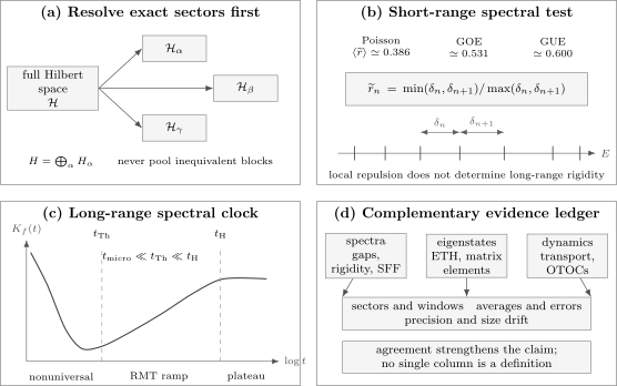
A many-body chaos claim is assembled in layers. Exact sectors must be separated before gap statistics are measured. Short-range repulsion does not fix the long-range form factor: the full form factor can contain smooth-density decay, while the connected random-matrix ramp begins only after a model-dependent Thouless time $t_{\rm Th}$ and saturates near the Heisenberg time $t_{\rm H}$. ETH and operator growth provide complementary, not interchangeable, evidence.

Thouless and Heisenberg Scales

Mean spacing and Heisenberg time

Let $\rho_\alpha(E)$ be the smooth density of states in the chosen sector. The local mean spacing is

$$\Delta_\alpha(E) = \frac{1}{ \rho_\alpha(E) }.$$

One common Heisenberg-time convention is

$$t_{\mathrm H}(E) = \frac{ 2\pi\hbar }{ \Delta_\alpha(E) } = 2\pi\hbar \rho_\alpha(E).$$

At finite energy density, with entropy measured in units of $k_{\mathrm B}$,

$$\rho_\alpha(E) \sim e^{S_\alpha(E)},$$

so

$$t_{\mathrm H} \sim \hbar e^{S_\alpha(E)}$$

up to algebraic and convention-dependent factors. The plateau is therefore exponentially late in system size for a many-body Hamiltonian.

Thouless time

The many-body Thouless time $t_{\mathrm{Th}}$ is the scale beyond which a chosen spectral diagnostic approaches its random-matrix prediction:

$$\begin{gathered} t \gtrsim t_{\mathrm{Th}} \\ \Longleftrightarrow \\ \text{RMT-like correlations} \\ \text{at the probed scale}. \end{gathered}$$

Its reciprocal defines a Thouless energy,

$$E_{\mathrm{Th}} \sim \frac{\hbar}{ t_{\mathrm{Th}} }.$$

The notation hides conventions. A value inferred from the connected spectral form factor need not match one inferred from number variance or observable matrix elements without order-one or even parametric differences.

The expected hierarchy in a developed chaotic regime is

$$t_{\mathrm{micro}} \ll t_{\mathrm{Th}} \ll t_{\mathrm H}.$$

If no interval separates $t_{\mathrm{Th}}$ and $t_{\mathrm H}$ at accessible sizes, a visible ramp may be too short to support a scaling claim.

Conserved densities and diffusion

Locality prevents conserved densities from relaxing instantly. For a diffusive mode,

$$\partial_t n(\mathbf x,t) = D\nabla^2 n(\mathbf x,t).$$

In a periodic box of linear size $L$, the slowest nonuniform mode has

$$q_{\min} = \frac{2\pi}{L},$$

and a relaxation time

$$\tau_{\mathrm{diff}} = \frac{1}{ Dq_{\min}^2 } = \frac{ L^2 }{ 4\pi^2D }.$$

In models where diffusion controls the onset of spectral universality,

$$t_{\mathrm{Th}} \sim \tau_{\mathrm{diff}}$$

up to definition-dependent factors. Ballistic, subdiffusive, anomalous, or constrained systems can scale differently. Energy conservation in a static Hamiltonian and charge conservation in a Floquet circuit need not produce identical form factors.

Dimensionless spectral window

A useful scale count is

$$g_{\mathrm{Th}} \sim \frac{ E_{\mathrm{Th}} }{ \Delta } \sim \frac{ t_{\mathrm H} }{ t_{\mathrm{Th}} },$$

where factors such as $2\pi$ depend on convention. Large $g_{\mathrm{Th}}$ means many levels lie inside the universal energy window.

The important lesson is directional:

$$\begin{gathered} \text{RMT is an infrared statement} \\ \text{in energy differences} \end{gathered}$$

or, equivalently, a late-time statement before the discrete-spectrum plateau. It does not say that a local Hamiltonian resembles a dense random matrix at microscopic energy scales.

Random Matrix Theory as an Effective Description

Random-matrix theory enters a local many-body problem as an effective theory of selected unfolded fluctuations, not as an entry-by-entry model of the Hamiltonian. A spin chain or lattice Hamiltonian remains sparse, local, and constrained by conservation laws even when its late, symmetry-resolved spectral correlations approach an invariant-ensemble benchmark.

The universal layer can include the Dyson class, short-range repulsion, long-range unfolded correlations, and a connected form-factor ramp and plateau. It does not determine the global density of states, hydrodynamic coefficients, quasiparticles, operator support, ETH envelopes, or microscopic relaxation times. Those nonuniversal structures set the Thouless scale and the window in which a random-matrix comparison is justified.

Random Matrix Theory in Quantum Matter derives the Gaussian and circular measures, Vandermonde repulsion, Wigner surmises, sine kernel, and symmetry-class extension. The present page retains the many-body applicability boundary, finite-size workflow, and dynamical interpretation.

Gaussian and circular ensembles

For a static Hamiltonian, one commonly compares bulk energies with the matching Gaussian class. For a periodic drive, the one-period unitary

$$U_F \lvert\phi_n\rangle = e^{-i\theta_n} \lvert\phi_n\rangle$$

has eigenphases $\theta_n$ on a circle. The natural benchmarks are circular orthogonal, unitary, or symplectic ensembles. Phase wrapping, exact quasienergy symmetries, and the absence of energy conservation change the many-body analysis.

Floquet Operators owns quasienergy kinematics, and Floquet Systems Preview owns heating and driven phase structure.

Spectral edges and special points

Bulk sine-kernel intuition should not be applied blindly to:

• the ground-state edge;
• a mobility edge;
• a symmetry-protected zero energy;
• a many-body phase transition;
• an exceptional point of a non-Hermitian generator;
• a quasienergy symmetry point at $0$ or $\pi$.

Edge statistics, chiral kernels, and non-Hermitian spectra require separate ensembles and scalings.

Benchmark Many-Body Settings

Mixed-field Ising chain

Consider an open spin chain

$$\begin{aligned} H &= -J \sum_{j=1}^{L-1} \sigma_j^z\sigma_{j+1}^z \\ &\quad - h_x \sum_{j=1}^{L} \sigma_j^x \\ &\quad - h_z \sum_{j=1}^{L} \sigma_j^z. \end{aligned}$$

At $h_z=0$, the transverse-field Ising chain maps to free fermions and is integrable. Generic nonzero $h_x$ and $h_z$ break that structure. With real couplings and a basis in which the Hamiltonian is real, an irreducible block typically compares with GOE statistics.

Open boundaries leave reflection symmetry when the fields are uniform. Pooling even and odd reflection sectors obscures repulsion. Edge fields can remove reflection symmetry, but they also change finite-size effects and must be declared.

XXZ chain with integrability breaking

A standard interpolation is

$$\begin{aligned} H(\lambda) &= J_1 \sum_j \left( S_j^xS_{j+1}^x + S_j^yS_{j+1}^y \right. \\ &\qquad\left. + \Delta_z S_j^zS_{j+1}^z \right) \\ &\quad + \lambda J_2 \sum_j \left( S_j^xS_{j+2}^x + S_j^yS_{j+2}^y \right. \\ &\qquad\left. + \Delta_2 S_j^zS_{j+2}^z \right). \end{aligned}$$

At an integrable point, symmetry-resolved bulk statistics are often approximately Poisson. Generic next-nearest-neighbor couplings produce a finite-size crossover toward Wigner–Dyson statistics.

The phrase “the crossover coupling” is incomplete unless it names:

• system size;
• magnetization and momentum sector;
• energy-density window;
• boundary conditions;
• chosen statistic;
• numerical threshold.

Different diagnostics can cross over at different apparent couplings.

Floquet circuits

Local random circuits and dual-unitary circuits provide analytically tractable laboratories. For a Floquet unitary,

$$K(t) = \left\langle \left| \operatorname{Tr} U_F^t \right|^2 \right\rangle, \qquad t\in\mathbb Z.$$

Special circuit ensembles admit exact mappings to classical partition functions or transfer matrices. They demonstrate that many-body random-matrix correlations can emerge without a semiclassical limit.

They are proofs for stated model classes, not proofs that every nonintegrable Hamiltonian has the same onset scale.

Relation to ETH

Shared regime, different statements

The ETH ansatz for a few-body observable $O$ has the schematic form

$$\begin{aligned} O_{mn} &= \overline O(E) \delta_{mn} \\ &\quad + e^{-S(E)/2} f_O(E,\omega) R_{mn}, \end{aligned}$$

with

$$E = \frac{E_m+E_n}{2}, \qquad \omega = E_m-E_n.$$

Spectral chaos concerns correlations among the $E_n$. ETH concerns matrix elements of a declared observable in the energy basis. The two data sets are not the same.

A generic nonintegrable parameter regime often exhibits both:

$$\begin{gathered} \text{Wigner–Dyson spectral correlations} \\ \text{and} \\ \text{ETH-like local matrix elements}. \end{gathered}$$

This is a powerful empirical pattern, not a biconditional theorem.

Random variables retain envelopes and correlations

The factor $R_{mn}$ is often modeled as a zero-mean unit-variance random variable over a local energy window. But locality, conservation, Hermiticity, and higher-point consistency impose correlations. The smooth envelope $f_O(E,\omega)$ contains dynamical information such as transport and spectral weight.

At low frequency, a conserved mode can produce structure that a featureless random matrix misses. Random-matrix behavior for matrix elements may emerge only below an observable-dependent frequency scale.

Counterexamples to naive equivalence

• A spectrum can have Wigner–Dyson statistics while a rare set of scarred states violates strong ETH.
• Hilbert-space fragmentation can support ETH-like behavior inside each large component while the union retains memory.
• A chosen local observable can look thermal in a model whose full spectral diagnostics are subtle.
• Mixing exact sectors can make a thermalizing model look Poisson.
• A localized or integrable model can show Poisson statistics for entirely different reasons.
• Spectral statistics alone do not determine a relaxation time or transport law.

Use spectral and ETH tests as mutually constraining evidence, not as synonyms.

OTOC and Scrambling Preview

For initially separated local operators $W_x$ and $V_0$, define

$$W_x(t) = e^{iHt/\hbar} W_x e^{-iHt/\hbar}$$

and a squared commutator

$$C(x,t) = \frac{1}{2} \left\langle [W_x(t),V_0]^\dagger [W_x(t),V_0] \right\rangle.$$

This probes whether the evolved operator has reached and become noncommuting with the probe at the origin. Spatially resolved $C(x,t)$ can reveal a butterfly front, broadening, and saturation.

It answers a different question from level statistics:

$$\begin{gathered} \text{level statistics} \longrightarrow \text{energy correlations}, \\ \text{OTOC} \longrightarrow \text{operator noncommutativity}, \\ \text{scrambling} \longrightarrow \\ \text{delocalization of} \\ \text{recoverable information}. \end{gathered}$$

Chaotic systems often show all three, but:

• integrable systems can have ballistic operator fronts;
• free systems can make selected OTOCs decay;
• random-matrix-like spectra do not determine spatial growth;
• a global OTOC can hide front geometry;
• finite-dimensional saturation can mimic a plateau.

Scrambling and OTOCs Preview supplies the regularized thermal correlators, velocity hierarchy, chaos-bound assumptions, and measurement protocols. Here the OTOC is only one independent column in the evidence ledger.

The SYK Model Preview gives a controlled all-to-all example in which an early large-$N$ Lyapunov window and much later parity-resolved random-matrix correlations coexist without being the same observable.

Eigenvectors and Basis Dependence

Let

$$\lvert E_n\rangle = \sum_a c_a^{(n)} \lvert a\rangle$$

in a chosen basis. The inverse participation ratio is

$$\operatorname{IPR}_n = \sum_a \left| c_a^{(n)} \right|^4.$$

An extended vector over $\mathcal D$ comparable components has

$$\operatorname{IPR} \sim \frac{1}{\mathcal D},$$

while a basis vector has $\operatorname{IPR}=1$.

This diagnostic is explicitly basis dependent. Delocalization in the computational basis can mean something different from delocalization in the eigenbasis of a nearby integrable Hamiltonian. Haar-random vector benchmarks also ignore energy locality and conservation laws unless the comparison ensemble is restricted appropriately.

Entanglement entropy, Porter–Thomas intensity statistics, participation entropies, and eigenstate correlations provide additional evidence. None alone defines chaos. Volume Laws owns the entanglement scaling of states.

A Reproducible Spectral Workflow

1. Specify the operator

Record the Hamiltonian or Floquet unitary, couplings, boundary conditions, system size, and numerical precision. Verify Hermiticity or unitarity.

2. Construct irreducible blocks

Identify every exact unitary and antiunitary symmetry. Check dimensions against independent state counting. Remove Kramers duplication correctly.

3. Select a bulk window

Use a fixed energy-density interval where the density is smooth and enough levels remain. Repeat with shifted and narrowed windows.

4. Inspect raw spectra

Look for unexplained exact degeneracies, duplicate states, solver failures, and sector contamination before applying statistics.

5. Compute local tests

Report the full $\widetilde r$ distribution, its mean, sample count, uncertainty, and size drift. If unfolded spacings are used, publish the unfolding method.

6. Compute long-range tests

Use number variance, rigidity, or a connected filtered spectral form factor. Vary filters and smoothing bandwidths.

7. Extract scales

Define the fitting criterion for $t_{\mathrm{Th}}$, $t_{\mathrm H}$, or $E_{\mathrm{Th}}$. Compare with transport times rather than assigning an interpretation from the symbol alone.

8. Add nonspectral evidence

Test ETH matrix elements, local relaxation, transport, entanglement, or operator growth as appropriate. State disagreements instead of averaging them away.

9. Scale the entire analysis

Increase $L$, compare adjacent symmetry sectors when theoretically appropriate, vary boundary conditions, and track the number of levels. A single mid-spectrum curve is an observation, not a thermodynamic conclusion.

Evidence Ledger

Evidence	Strong observation	What it does not establish
adjacent-gap ratios	local repulsion in one block	long-range rigidity or ETH
spacing distribution	Dyson small-$s$ exponent	mechanism or universal window
number variance	rigidity across many levels	dynamics of local observables
connected form factor	ramp and plateau after declared averaging	spatial scrambling
ETH matrix elements	thermal smoothness and entropy scaling	complete RMT independence
participation statistics	basis-relative delocalization	locality or thermalization
OTOC front	spatial operator growth	spectral universality
local relaxation	loss of memory for chosen observables	absence of scars or hidden sectors
size scaling	stability or systematic drift	the infinite-size limit without a model

The strongest case is overdetermined: several columns agree after their assumptions and scales are made compatible.

Finite-Size and Numerical Failure Modes

Exponentially small spacings

In a bulk sector,

$$\Delta(E) \sim e^{-s(e)L}$$

up to powers of $L$. Numerical eigenvalue errors must be much smaller than the spacings being analyzed. Loss of orthogonality, insufficient solver tolerance, or accidental duplicate eigenpairs can distort the smallest gaps first.

Too few levels after symmetry resolution

Correctly resolving symmetries reduces matrix dimension. A very small block may not support a stable histogram. Pooling inequivalent blocks to increase statistics solves the sample-size problem by changing the physical ensemble, which is not acceptable.

Equivalent sectors related by an exact unitary mapping may be averaged only after demonstrating their equivalence and removing duplicate eigenvalues.

Edge contamination

The low-energy edge can retain quasiparticles, broken-symmetry towers, topology, or critical scaling even when the middle of the spectrum is chaotic. State the energy density and do not generalize a mid-spectrum result to the ground state.

Polynomial unfolding artifacts

A high-order fit can absorb genuine rigidity, while a low-order fit can leave curvature. Gap ratios, several unfolding schemes, and filtered form factors should be compared.

Disorder and sample averages

Disorder averaging can conceal broad sample-to-sample distributions. Report medians or quantiles when rare samples matter. Do not treat neighboring levels from one realization as fully independent observations.

Dense versus partial eigensolvers

Shift-invert methods can target a spectral window, but spectral transformation and finite tolerance require validation against dense diagonalization at smaller $L$. Missing or duplicated states invalidate spacing statistics even if individual eigenvalues look accurate.

Experimental Access

Direct many-body spectroscopy becomes exponentially demanding, so experiments often probe adjacent ideas rather than reconstructing a macroscopic spectrum.

Controllable few-qubit systems can map eigenphases, reconstruct states, and compare ergodic and regular parameter regions. Larger quantum processors can measure OTOCs, operator spreading, randomized observables, return probabilities, or spectral form factors through interferometric and randomized protocols.

Experimental claims need an expanded ledger:

• finite coherence time and gate error;
• imperfect symmetry conservation;
• state-preparation and measurement bias;
• ensemble or random-circuit averaging;
• classical postprocessing assumptions;
• accessible time relative to $t_{\mathrm{Th}}$ and $t_{\mathrm H}$;
• comparison with calibrated integrable and chaotic controls.

Observing rapid entanglement growth or OTOC decay is valuable evidence for information spreading. It is not a direct measurement of Wigner–Dyson energy statistics unless the protocol explicitly reconstructs the relevant spectral correlator.

Boundaries with Neighboring Phenomena

Integrability

Integrability is positive structure: an extensive controlled family of charges, factorized scattering, transfer matrices, or equivalent exact machinery. Poisson statistics is supportive evidence after symmetry resolution, not the definition.

Many-body localization

MBL phenomenology combines Poisson-like spectra with local memory, nonthermal eigenstates, suppressed transport, and characteristic entanglement dynamics. Poisson statistics alone cannot distinguish it from a clean integrable model or sector mixing.

Prethermalization

A prethermal system can show chaotic dynamics within an approximately conserved sector while drifting only slowly between sectors. The relevant random-matrix block can therefore be defined by dressed quasi-conserved quantities over an intermediate time window.

Quantum scars

A sparse set of atypical eigenstates can coexist with a mostly Wigner–Dyson spectrum and weak ETH. Special initial states can revive even when typical states thermalize. Bulk spectral chaos does not erase every structured eigenstate.

Hydrodynamics

Hydrodynamic modes are not failures of chaos. They are universal consequences of conservation and locality that control relaxation before the pure random-matrix regime. Calling every slow mode “nonergodic” confuses a transport timescale with asymptotic memory.

Open systems

Liouvillian and non-Hermitian spectra have complex eigenvalues and different symmetry classifications. Hermitian spacing ratios and Gaussian ensembles cannot be transferred unchanged.

Common Mistakes

• Pooling particle-number, momentum, parity, spin, or gauge sectors.
• Checking time-reversal symmetry of the full Hamiltonian instead of its action within one block.
• Leaving Kramers zero spacings in a GSE comparison.
• Treating the Wigner surmise as the exact large-matrix spacing distribution.
• Quoting a gap-ratio mean without the energy window, sample count, uncertainty, or system size.
• Claiming that gap ratios require no density or edge checks because they avoid explicit unfolding.
• Inferring long-range rigidity from nearest-neighbor repulsion.
• Plotting an unconnected spectral form factor and labeling density-of-states decay a universal dip.
• Extracting a Thouless time without a fitting criterion or competing transport scale.
• Equating spectral chaos with ETH, thermalization, operator growth, or scrambling.
• Calling Poisson statistics proof of integrability or localization.
• Comparing a static Hamiltonian spectrum with a circular ensemble, or Floquet eigenphases with a Gaussian ensemble, without justification.
• Ignoring solver precision when spacings are exponentially small.
• Treating one finite-size crossover as a thermodynamic phase boundary.
• Using eigenvector delocalization without naming the basis.

Worked Microexamples

Mixed symmetry sectors

Suppose

$$H = H_+\oplus H_-,$$

where each parity block has GOE-like statistics. A level $E_m^+$ can cross a level $E_n^-$ because parity forbids coupling:

$$\langle E_m^+|H|E_n^-\rangle = 0.$$

The merged sequence contains many unconstrained cross-sector spacings. Its small-$s$ distribution can have nonzero weight even though each block separately repels. The correct conclusion is not “the model is integrable,” but “the pooled spectrum is not an irreducible ensemble.”

Poisson gap-ratio law

For independent exponential gaps $x$ and $y$ with unit mean, define

$$r = \frac{\min(x,y)}{\max(x,y)}.$$

The ratio density on $0\le r\le1$ is

$$p_{\mathrm P}(r) = \frac{2}{ (1+r)^2 }.$$

Its mean is

$$\begin{aligned} \langle r\rangle_{\mathrm P} &= 2 \int_0^1 \frac{r\,dr}{ (1+r)^2 } \\ &= 2\ln2-1. \end{aligned}$$

The derivation appears as an exercise below and illustrates why no unfolding is needed for this local ratio.

Exponential separation of spectral times

If a sector contains

$$\mathcal D_\alpha \sim e^{sL}$$

states in a fixed-width bulk band, then

$$\Delta \sim e^{-sL}$$

and

$$t_{\mathrm H} \sim e^{sL}.$$

If diffusion sets

$$t_{\mathrm{Th}} \sim L^2,$$

then

$$\frac{ t_{\mathrm H} }{ t_{\mathrm{Th}} } \sim \frac{ e^{sL} }{ L^2 }.$$

The universal spectral window can contain exponentially many levels even though it starts only after a polynomially long hydrodynamic time.

Exercises

1. Derive the Poisson adjacent-gap ratio

Let $x$ and $y$ be independent exponentially distributed gaps with density $e^{-x}$ for $x\ge0$. Derive the probability density and mean of

$$r = \frac{\min(x,y)}{\max(x,y)}.$$

Solution

By symmetry, restrict to $0<x<y$ and multiply by two. Insert a delta function:

$$\begin{aligned} p(r) &= 2 \int_0^\infty dy \\ &\quad\times \int_0^y dx\, e^{-x-y} \delta\left( r-\frac{x}{y} \right). \end{aligned}$$

Using

$$\delta\left( r-\frac{x}{y} \right) = y\, \delta(x-ry),$$

gives

$$\begin{aligned} p(r) &= 2 \int_0^\infty y e^{-(1+r)y}\,dy \\ &= \frac{2}{ (1+r)^2 }, \qquad 0\le r\le1. \end{aligned}$$

It is normalized because

$$\int_0^1 \frac{2\,dr}{ (1+r)^2 } = 1.$$

For the mean,

$$\begin{aligned} \langle r\rangle &= 2 \int_0^1 \frac{r\,dr}{ (1+r)^2 } \\ &= 2 \left[ \ln(1+r) + \frac{1}{1+r} \right]_0^1 \\ &= 2\ln2-1. \end{aligned}$$

2. Normalize the GOE Wigner surmise

Show that

$$P(s) = \frac{\pi}{2} s e^{-\pi s^2/4}$$

is normalized and has unit mean spacing.

Solution

For $a>0$,

$$\int_0^\infty s e^{-as^2}\,ds = \frac{1}{2a}.$$

With $a=\pi/4$,

$$\int_0^\infty P(s)\,ds = \frac{\pi}{2} \frac{1}{ 2(\pi/4) } = 1.$$

Also,

$$\int_0^\infty s^2e^{-as^2}\,ds = \frac{\sqrt{\pi}}{ 4a^{3/2} }.$$

Therefore

$$\begin{aligned} \langle s\rangle &= \frac{\pi}{2} \frac{\sqrt{\pi}}{ 4(\pi/4)^{3/2} } \\ &= 1. \end{aligned}$$

The result verifies the chosen normalization. It does not make the surmise the exact large-GOE distribution.

3. Resolve a translation and time-reversal subtlety

A periodic spin chain has time-reversal symmetry and translation symmetry. Explain why a generic momentum block $k$ can display GUE statistics while the $k=0$ block displays GOE statistics, assuming $\Theta^2=+I$ and no other antiunitary operation acts within the generic block.

Solution

Time reversal reverses momentum:

$$\Theta: \mathcal H_k \longrightarrow \mathcal H_{-k}.$$

For generic $k$, the sectors $k$ and $-k$ are distinct. Thus $\Theta$ is a symmetry of their direct sum but is not an antiunitary operator acting inside $\mathcal H_k$. The irreducible $k$ block therefore has no internal antiunitary constraint and can belong to the unitary class.

At $k=0$, one has $-k=k$ modulo the reciprocal lattice vector. Time reversal acts within the block and squares to $+I$, selecting the orthogonal class after any remaining unitary symmetries are resolved.

Pooling $k$ and $-k$ to “restore” time reversal is not a GOE analysis; it combines two correlated but distinct blocks.

4. Avoided crossing criterion

Diagonalize

$$H(\lambda) = \begin{pmatrix} a\lambda & v \\ v^* & -a\lambda \end{pmatrix}$$

and find its minimum level spacing. What changes if a symmetry forces $v=0$?

Solution

The characteristic equation is

$$E^2 = a^2\lambda^2+|v|^2,$$

so

$$E_\pm = \pm \sqrt{ a^2\lambda^2+|v|^2 }.$$

The spacing is

$$E_+-E_- = 2 \sqrt{ a^2\lambda^2+|v|^2 },$$

with minimum

$$\Delta E_{\min} = 2|v|$$

at $\lambda=0$.

If symmetry forces $v=0$, then

$$E_\pm = \pm|a\lambda|,$$

and the levels cross exactly at $\lambda=0$. This is the local reason independent symmetry sectors must not be pooled in a repulsion test.

5. Compare Thouless and Heisenberg times

Assume a one-dimensional diffusive chaotic chain has entropy density $s$, diffusion constant $D$ independent of $L$, and a fixed-width bulk spectral window. Estimate the size dependence of $t_{\mathrm{Th}}$, $t_{\mathrm H}$, and their ratio.

Solution

The slowest diffusive wave number is

$$q_{\min} = \frac{2\pi}{L}.$$

Hence

$$t_{\mathrm{Th}} \sim \frac{1}{ Dq_{\min}^2 } \sim \frac{L^2}{D},$$

where an order-one geometric factor has been suppressed.

The number of states in the bulk window scales as

$$\mathcal D \sim e^{sL},$$

so the mean spacing scales as

$$\Delta \sim e^{-sL}.$$

Therefore

$$t_{\mathrm H} \sim \frac{\hbar}{\Delta} \sim \hbar e^{sL}.$$

The ratio is

$$\frac{ t_{\mathrm H} }{ t_{\mathrm{Th}} } \sim \frac{ \hbar D e^{sL} }{ L^2 }.$$

Thus the interval between hydrodynamic relaxation and spectral discreteness grows rapidly with $L$, even though direct numerical access to $t_{\mathrm H}$ becomes correspondingly difficult.

6. Why the connected form factor is needed

Suppose the averaged filtered amplitude is nonzero:

$$\left\langle Z_f(t)\right\rangle \ne 0.$$

Show how the ordinary form factor decomposes and explain what the disconnected term measures.

Solution

Write

$$Z_f(t) = \left\langle Z_f(t)\right\rangle + \delta Z_f(t),$$

with

$$\left\langle \delta Z_f(t) \right\rangle = 0.$$

Then

$$\begin{aligned} \left\langle \left| Z_f(t) \right|^2 \right\rangle &= \left| \left\langle Z_f(t) \right\rangle \right|^2 \\ &\quad + \left\langle \left| \delta Z_f(t) \right|^2 \right\rangle. \end{aligned}$$

The first term is the disconnected piece. It is controlled by the smooth one-level density and the chosen filter. The second term is

$$K_{f,\mathrm c}(t) = \left\langle \left| \delta Z_f(t) \right|^2 \right\rangle,$$

which probes connected spectral fluctuations. Failing to subtract the first term can confuse the Fourier transform of the density of states with two-level universality.

7. Distinguish spectral chaos from ETH

A model has GOE-like gap ratios in the middle of each symmetry sector, but one specially prepared product state shows long-lived revivals. List three logically different explanations and one diagnostic for each.

Solution

Possible explanations include:

1. Quantum scars. A sparse set of atypical eigenstates has large overlap with the product state. Inspect overlap weights, eigenstate entanglement, and diagonal matrix elements of the participating states.
2. Approximate conservation or prethermalization. The state lies in an almost-invariant manifold. Track a proposed quasi-conserved quantity and scale the revival or plateau lifetime with the symmetry-breaking parameter.
3. Finite-size recurrence. A small set of commensurate gaps produces a revival. Increase $L$, vary boundaries, and test whether the recurrence time and amplitude drift.

One could also test sector contamination, an exact dynamical symmetry, or fragmentation. GOE-like bulk spacings rule out none of these state-selective mechanisms by themselves.

8. Design a converged spin-chain test

Design a numerical test of the integrability-to-chaos crossover in the mixed-field Ising chain. Your answer must specify sectors, windows, local and long-range diagnostics, and a finite-size check.

Solution

A defensible design is:

1. Choose open boundaries and fixed $J$ and $h_x$, then scan $h_z$ from zero into a generic nonintegrable regime.
2. Resolve reflection parity for uniform open chains. If edge fields break reflection, document them and analyze the resulting single block.
3. For each $L$, choose one or more fixed central energy-density windows and exclude the spectral edges.
4. Compute the full adjacent-gap-ratio distribution and mean with a bootstrap uncertainty.
5. Independently unfold with at least two smooth-density procedures and compare the spacing distribution and number variance.
6. Compute a filtered connected spectral form factor, varying the filter and smoothing bandwidth.
7. Extract crossover couplings separately for each diagnostic rather than assuming one value.
8. Repeat over several $L$ and shifted windows. Validate partial eigensolver output against dense diagonalization at smaller sizes.
9. Compare with ETH diagonal fluctuations for a local observable, while keeping that result conceptually separate from the spectral tests.

The output should report drift and uncertainty, not only the visually best collapse.

Status Ledger

Established within stated settings

• Dyson symmetry classes organize bulk spectral correlations after irreducible sector resolution.
• Local repulsion and long-range rigidity are distinct observables.
• Exact or asymptotically controlled random-matrix form-factor results occur in special solvable many-body circuits and driven models.
• Conserved modes can control the onset of the random-matrix ramp.

Model dependent

• The crossover strength away from integrability;
• the scaling and even the operational definition of $t_{\mathrm{Th}}$;
• the relation between spectral onset and transport or scrambling times;
• the size of the energy window over which RMT applies;
• the quality of eigenvector random-matrix statistics.

Active frontier

• Generic derivations for deterministic finite-range Hamiltonians;
• higher-order spectral and eigenstate correlations beyond pairwise ETH;
• controlled extrapolation from accessible exact-diagonalization sizes;
• robust spectral-form-factor protocols on large quantum devices;
• universality across all Dyson classes and conserved-mode structures.

Recent analytic work continues to extend spectral-form-factor calculations across symmetry classes in periodically kicked interacting systems. Those results strengthen a program, not a theorem covering all local many-body Hamiltonians.

Key Takeaways

• Many-body quantum chaos is diagnosed by a family of scale- and symmetry-aware tests.
• Exact symmetry resolution comes before every spacing or form-factor calculation.
• Gap ratios are convenient local probes, not substitutes for long-range statistics or finite-size analysis.
• Random-matrix universality concerns fluctuations below a Thouless energy, not microscopic matrix entries or global density of states.
• $t_{\mathrm{Th}}$ marks the onset of a universal regime; $t_{\mathrm H}$ resolves discreteness and is typically exponentially larger.
• ETH, spectral chaos, eigenvector delocalization, and scrambling are deeply related but not equivalent.
• Conserved hydrodynamic modes delay universal spectral behavior without disproving chaos.
• The most trustworthy conclusion is overdetermined and reports all averaging, windows, uncertainties, and size drift.

Further Connections

• Relaxation and Thermalization for dephasing, equilibration, and ensemble selection;
• Exact Solutions Preview for positive criteria of integrability;
• Time-Dependent Correlations for ordinary dynamical correlators and spectral functions;
• Number Operators and Conserved Quantities for symmetry-sector construction;
• Microcanonical Ensemble for energy-window conventions.
• SYK Model Preview for a model-specific mod-8 symmetry cycle, disorder average, and finite-$N$ benchmark.

References

• F. J. Dyson, “The threefold way: algebraic structure of symmetry groups and ensembles in quantum mechanics,” Journal of Mathematical Physics 3, 1199–1215 (1962). doi:10.1063/1.1703863
• M. L. Mehta, Random Matrices, 3rd ed., Elsevier (2004).
• F. Haake, Quantum Signatures of Chaos, 3rd ed., Springer (2010).
• M. V. Berry and M. Tabor, “Level clustering in the regular spectrum,” Proceedings of the Royal Society A 356, 375–394 (1977). doi:10.1098/rspa.1977.0140
• O. Bohigas, M. J. Giannoni, and C. Schmit, “Characterization of chaotic quantum spectra and universality of level fluctuation laws,” Physical Review Letters 52, 1–4 (1984). doi:10.1103/PhysRevLett.52.1
• D. A. Rabson, B. N. Narozhny, and A. J. Millis, “Crossover from Poisson to Wigner–Dyson level statistics in spin chains with integrability breaking,” Physical Review B 69, 054403 (2004). doi:10.1103/PhysRevB.69.054403
• V. Oganesyan and D. A. Huse, “Localization of interacting fermions at high temperature,” Physical Review B 75, 155111 (2007). doi:10.1103/PhysRevB.75.155111
• L. F. Santos and M. Rigol, “Onset of quantum chaos in one-dimensional bosonic and fermionic systems and its relation to thermalization,” Physical Review E 81, 036206 (2010). doi:10.1103/PhysRevE.81.036206
• Y. Y. Atas, E. Bogomolny, O. Giraud, and G. Roux, “Distribution of the ratio of consecutive level spacings in random matrix ensembles,” Physical Review Letters 110, 084101 (2013). doi:10.1103/PhysRevLett.110.084101
• L. D’Alessio, Y. Kafri, A. Polkovnikov, and M. Rigol, “From quantum chaos and eigenstate thermalization to statistical mechanics and thermodynamics,” Advances in Physics 65, 239–362 (2016). doi:10.1080/00018732.2016.1198134
• P. Kos, M. Ljubotina, and T. Prosen, “Many-body quantum chaos: analytic connection to random matrix theory,” Physical Review X 8, 021062 (2018). doi:10.1103/PhysRevX.8.021062
• B. Bertini, P. Kos, and T. Prosen, “Exact spectral form factor in a minimal model of many-body quantum chaos,” Physical Review Letters 121, 264101 (2018). doi:10.1103/PhysRevLett.121.264101
• A. Chan, A. De Luca, and J. T. Chalker, “Spectral statistics in spatially extended chaotic quantum many-body systems,” Physical Review Letters 121, 060601 (2018). doi:10.1103/PhysRevLett.121.060601
• A. Chan, A. De Luca, and J. T. Chalker, “Solution of a minimal model for many-body quantum chaos,” Physical Review X 8, 041019 (2018). doi:10.1103/PhysRevX.8.041019
• H. Gharibyan, M. Hanada, S. H. Shenker, and M. Tezuka, “Onset of random matrix behavior in scrambling systems,” Journal of High Energy Physics 2018, 124 (2018). doi:10.1007/JHEP07(2018)124
• A. J. Friedman, A. Chan, A. De Luca, and J. T. Chalker, “Spectral statistics and many-body quantum chaos with conserved charge,” Physical Review Letters 123, 210603 (2019). doi:10.1103/PhysRevLett.123.210603
• A. Chan, A. De Luca, and J. T. Chalker, “Eigenstate correlations, thermalization, and the butterfly effect,” Physical Review Letters 122, 220601 (2019). doi:10.1103/PhysRevLett.122.220601
• L. Foini and J. Kurchan, “Eigenstate thermalization hypothesis and out of time order correlators,” Physical Review E 99, 042139 (2019). doi:10.1103/PhysRevE.99.042139
• M. Winer and B. Swingle, “Hydrodynamic theory of the connected spectral form factor,” Physical Review X 12, 021009 (2022). doi:10.1103/PhysRevX.12.021009
• A. Dymarsky, “Bound on eigenstate thermalization from transport,” Physical Review Letters 128, 190601 (2022). doi:10.1103/PhysRevLett.128.190601
• C. Neill et al., “Ergodic dynamics and thermalization in an isolated quantum system,” Nature Physics 12, 1037–1041 (2016). doi:10.1038/nphys3830
• X. Mi et al., “Information scrambling in computationally complex quantum circuits,” Science 374, 1479–1483 (2021). doi:10.1126/science.abg5029
• V. Kumar, T. Prosen, and D. Roy, “Leading and beyond leading-order spectral form factor in chaotic quantum many-body systems across all Dyson symmetry classes,” Physical Review X, accepted 21 May 2026. doi:10.1103/kwh6-hncn