Microcanonical Ensemble

The microcanonical ensemble represents an isolated quantum system whose exact conserved quantities are fixed and whose energy is restricted to a specified shell. For a fixed-particle-number Hamiltonian $H_N$, choose the interval

$$I_{E,\Delta E} = \left[ E-\frac{\Delta E}{2}, E+\frac{\Delta E}{2} \right].$$

Let

$$\Pi_{E,\Delta E} = \mathbf 1_{I_{E,\Delta E}}(H_N)$$

be the spectral projector onto that interval. If

$$W(E,\Delta E,N,V) = \operatorname{Tr}_{\mathcal H_N} \Pi_{E,\Delta E}$$

is finite and nonzero, the microcanonical density operator is

$$\rho_{\mathrm{mc}} = \frac{ \Pi_{E,\Delta E} }{ W(E,\Delta E,N,V) }.$$

This page is the canonical home for quantum energy shells, their state counts, microcanonical entropy, thermodynamic derivatives, and their qualified relation to isolated-system dynamics.

The Energy-Shell Projector

Suppose the Hamiltonian has spectral resolution

$$H_N = \sum_a E_aP_a,$$

where $P_a$ projects onto the eigenspace of energy $E_a$. Then

$$\Pi_{E,\Delta E} = \sum_{E_a\in I_{E,\Delta E}} P_a.$$

If

$$g_a = \operatorname{Tr}P_a$$

is the degeneracy of $E_a$, the shell dimension is

$$W = \sum_{E_a\in I_{E,\Delta E}} g_a.$$

The microcanonical state therefore assigns equal weight per orthonormal state inside the shell:

$$\rho_{\mathrm{mc}} = \frac{1}{W} \sum_{E_a\in I_{E,\Delta E}} P_a.$$

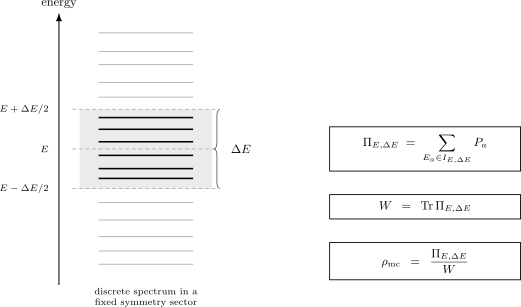
A finite quantum spectrum is restricted to a window of width $\Delta E$. The spectral projector retains every eigenspace in the window, $W=\operatorname{Tr}\Pi_{E,\Delta E}$ counts its dimension, and $\rho_{\mathrm{mc}}=\Pi_{E,\Delta E}/W$ is uniform on that subspace.

Basic Density-Operator Properties

Because $\Pi_{E,\Delta E}$ is an orthogonal projector,

$$\Pi_{E,\Delta E}^\dagger = \Pi_{E,\Delta E}, \qquad \Pi_{E,\Delta E}^2 = \Pi_{E,\Delta E}.$$

It follows that $\rho_{\mathrm{mc}}$ is Hermitian and positive. Its trace is

$$\operatorname{Tr}\rho_{\mathrm{mc}} = \frac{\operatorname{Tr}\Pi_{E,\Delta E}}{W} = 1.$$

Its support is exactly the energy-shell subspace:

$$\Pi_{E,\Delta E} \rho_{\mathrm{mc}} = \rho_{\mathrm{mc}}.$$

Within that support, all nonzero eigenvalues of $\rho_{\mathrm{mc}}$ are $1/W$. Therefore

$$\operatorname{rank}\rho_{\mathrm{mc}} = W,$$

and its purity is

$$\operatorname{Tr}\rho_{\mathrm{mc}}^2 = \frac{1}{W}.$$

The state is pure only when $W=1$.

Microcanonical Expectation Values

For an observable $A$,

$$\langle A\rangle_{\mathrm{mc}} = \operatorname{Tr} \left( \rho_{\mathrm{mc}}A \right) = \frac{1}{W} \operatorname{Tr} \left( \Pi_{E,\Delta E}A \right).$$

In the energy basis,

$$\langle A\rangle_{\mathrm{mc}} = \frac{1}{W} \sum_{E_a\in I_{E,\Delta E}} \operatorname{Tr} \left( P_aA \right).$$

Off-diagonal matrix elements between distinct energy eigenspaces do not contribute to this equilibrium average. Degenerate eigenspaces are included through their full projectors, so the formula is basis independent inside each degeneracy.

Energy Support and Fluctuations

Every energy in the shell lies between

$$E_- = E-\frac{\Delta E}{2}$$

and

$$E_+ = E+\frac{\Delta E}{2}.$$

Consequently,

$$E_- \leq \langle H_N\rangle_{\mathrm{mc}} \leq E_+.$$

The energy is not necessarily one exact eigenvalue. Its variance satisfies the support bound

$$\operatorname{Var}_{\mathrm{mc}}(H_N) \leq \frac{(\Delta E)^2}{4}.$$

Thus “fixed energy” means fixed to the declared shell. If the shell contains several eigenvalues, an energy measurement still has a distribution over those values.

Exact-Energy Special Case

If the energy is known exactly and $E_a$ is an eigenvalue, use

$$\Pi_{E_a} = P_a.$$

The exact-energy microcanonical state is

$$\rho_{E_a} = \frac{P_a}{g_a}.$$

For a nondegenerate eigenvalue,

$$g_a=1,$$

so

$$\rho_{E_a} = |E_a\rangle\langle E_a|$$

is pure. For a degenerate eigenvalue, the exact-energy ensemble is maximally mixed within the degenerate eigenspace unless further conserved quantities or preparation information resolve it.

This distinction matters in small systems. A single nondegenerate eigenstate has no large state count from which smooth thermodynamics can be inferred.

How Wide Should the Shell Be?

The shell width is part of the ensemble definition. A useful many-body window should be:

1. broad compared with the local level spacing;
2. narrow compared with the macroscopic energy scale;
3. stable under modest changes of its center and width;
4. restricted to the correct symmetry and conserved-charge sector.

Schematically, one wants

$$\delta E_{\mathrm{level}} \ll \Delta E \ll E_{\mathrm{macro}}.$$

Along a thermodynamic sequence, a common requirement is

$$W(E,\Delta E) \longrightarrow \infty$$

while

$$\frac{\Delta E}{E} \longrightarrow 0.$$

The two limits are compatible because the many-body level spacing often becomes extremely small as system size grows.

There is no universal shell width that works for every Hamiltonian, energy, and observable. Near spectral edges, gaps, mobility edges, first-order coexistence, or sparse symmetry sectors, the required checks can be especially delicate.

State Counting and Density of States

Define the cumulative state count

$$\Gamma_N(E) = \operatorname{Tr}_{\mathcal H_N} \Theta(E-H_N).$$

For a discrete spectrum, $\Gamma_N(E)$ is a staircase. Its distributional derivative is the density of states

$$\omega_N(E) = \operatorname{Tr}_{\mathcal H_N} \delta(E-H_N).$$

The shell count is

$$\begin{aligned} W(E,\Delta E) ={}& \Gamma_N \left( E+\frac{\Delta E}{2} \right) \\ &- \Gamma_N \left( E-\frac{\Delta E}{2} \right). \end{aligned}$$

If a coarse-grained density of states varies slowly across the window,

$$W(E,\Delta E) \simeq \omega_N(E)\Delta E.$$

For a finite exact spectrum, $\omega_N(E)$ is a sum of delta functions. Differentiating or taking logarithms therefore requires a shell, smoothing prescription, or thermodynamic limit. The Green Functions and Density of States page owns spectral-density methods; here the density of states is used for thermodynamic counting.

Microcanonical Entropy

The shell entropy is

$$S_{\mathrm{sh}}(E,\Delta E,N,V) = k_{\mathrm B}\ln W(E,\Delta E,N,V).$$

Because $W$ is dimensionless, the logarithm is well defined.

The von Neumann entropy of the microcanonical density operator gives the same result:

$$\begin{aligned} S_{\mathrm{vN}} \left( \rho_{\mathrm{mc}} \right) &= -k_{\mathrm B} \operatorname{Tr} \left( \rho_{\mathrm{mc}} \ln\rho_{\mathrm{mc}} \right) \\ &= k_{\mathrm B}\ln W. \end{aligned}$$

This equality relies on the uniform nonzero eigenvalues $1/W$.

Entropy Conventions

Several related quantities are called microcanonical entropy.

Shell-count entropy

The finite-window definition is

$$S_{\mathrm{sh}} = k_{\mathrm B}\ln W(E,\Delta E).$$

It makes the energy resolution explicit and is the primary convention on this page.

Density-of-states entropy

For a smoothed density of states, one may define

$$S_{\omega}(E) = k_{\mathrm B} \ln \left[ \omega(E)\varepsilon_0 \right],$$

where the reference energy $\varepsilon_0$ makes the logarithm dimensionless.

When $\omega(E)$ is nearly constant across the shell,

$$S_{\mathrm{sh}} \simeq S_\omega +k_{\mathrm B} \ln \left( \frac{\Delta E}{\varepsilon_0} \right).$$

Cumulative-count entropy

Another convention is

$$S_{\Gamma}(E) = k_{\mathrm B}\ln\Gamma(E).$$

For regular macroscopic systems, these definitions can share the same leading extensive entropy while differing by subextensive or finite-size terms. For small systems, bounded spectra, and questions about negative temperature, their derivatives can differ qualitatively.

Always state the convention before quoting a microcanonical temperature or heat capacity.

Maximum-Entropy Characterization

The microcanonical state is the maximum-entropy state supported in the chosen shell.

Let $\sigma$ be any density operator satisfying

$$\sigma = \Pi_{E,\Delta E} \sigma \Pi_{E,\Delta E}.$$

The quantum relative entropy is

$$D \left( \sigma \middle\| \rho_{\mathrm{mc}} \right) \geq 0.$$

On the shell,

$$\ln\rho_{\mathrm{mc}} = -\ln W.$$

Therefore

$$\begin{aligned} D \left( \sigma \middle\| \rho_{\mathrm{mc}} \right) &= \operatorname{Tr} \left( \sigma\ln\sigma \right) +\ln W \\ &= -\frac{S(\sigma)}{k_{\mathrm B}} +\ln W. \end{aligned}$$

Hence

$$S(\sigma) \leq k_{\mathrm B}\ln W,$$

with equality only for

$$\sigma = \rho_{\mathrm{mc}}.$$

Equal shell weights are thus a precise maximum-entropy assignment under a support constraint. This inference statement should not be confused with a proof that unitary dynamics randomizes amplitudes. Maximum Entropy Principle compares this exact-support problem with mean-value constraints and general exponential states.

Thermodynamic Temperature

Temperature is derived in the microcanonical ensemble. Let

$$\sigma(E,V,N) \equiv \frac{S(E,V,N)}{k_{\mathrm B}}$$

be a smooth dimensionless thermodynamic entropy. The inverse temperature is

$$\beta_{\mathrm{mc}} = \left( \frac{\partial\sigma}{\partial E} \right)_{V,N} = \frac{1}{k_{\mathrm B}} \left( \frac{\partial S}{\partial E} \right)_{V,N}.$$

Equivalently,

$$\frac{1}{T} = \left( \frac{\partial S}{\partial E} \right)_{V,N}.$$

This derivative presupposes a smooth entropy. For a finite staircase count, one must specify finite differences, interpolation, smoothing, or a limiting sequence.

Pressure and Chemical Potential

The microcanonical entropy representation has differential

$$dS = \frac{1}{T}dE +\frac{P}{T}dV -\frac{\mu}{T}dN.$$

Thus

$$\frac{P}{T} = \left( \frac{\partial S}{\partial V} \right)_{E,N},$$

and

$$-\frac{\mu}{T} = \left( \frac{\partial S}{\partial N} \right)_{E,V}.$$

Because $N$ is discrete in a finite quantum system, particle-addition derivatives are often implemented as finite differences. The thermodynamic chemical potential emerges after a suitable large-system limit.

Heat Capacity and Entropy Curvature

At fixed $V$ and $N$,

$$\frac{1}{T} = \frac{\partial S}{\partial E}.$$

Differentiating gives

$$-\frac{1}{T^2} \frac{\partial T}{\partial E} = \frac{\partial^2S}{\partial E^2}.$$

Therefore the microcanonical heat capacity is

$$C_{V,N} = \left( \frac{\partial E}{\partial T} \right)_{V,N} = -\frac{1}{ T^2 \left( \partial^2S/\partial E^2 \right)_{V,N} }.$$

In terms of the dimensionless entropy,

$$\frac{C_{V,N}}{k_{\mathrm B}} = -\frac{ \beta_{\mathrm{mc}}^2 }{ \left( \partial^2\sigma/\partial E^2 \right)_{V,N} }.$$

A concave entropy has

$$\frac{\partial^2S}{\partial E^2} < 0,$$

and therefore positive heat capacity. Convex regions can produce negative microcanonical heat capacity. Such behavior requires careful interpretation and may occur in finite systems with interface effects or in nonadditive long-range systems, where canonical and microcanonical descriptions can be nonequivalent.

Why Equal Temperatures Describe Equilibrium

Consider two weakly coupled systems $A$ and $B$ with fixed total energy

$$E_{\mathrm{tot}} = E_A+E_B.$$

The number of compatible states near a division $E_A$ is proportional to

$$W_A(E_A) W_B(E_{\mathrm{tot}}-E_A).$$

Its logarithm is

$$\frac{S_{\mathrm{tot}}(E_A)}{k_{\mathrm B}} = \frac{S_A(E_A)}{k_{\mathrm B}} +\frac{ S_B(E_{\mathrm{tot}}-E_A) }{ k_{\mathrm B} }.$$

At the most probable energy division,

$$\frac{dS_{\mathrm{tot}}}{dE_A} = 0.$$

Therefore

$$\left( \frac{\partial S_A}{\partial E_A} \right) = \left( \frac{\partial S_B}{\partial E_B} \right),$$

which gives

$$T_A = T_B.$$

Temperature is the quantity that equalizes because it is derived from the slope of entropy with respect to exchanged energy.

Connection to the Canonical Ensemble

The canonical partition function can be written as a transform of the density of states:

$$Z_N(\beta) = \int dE\, \omega_N(E) e^{-\beta E}.$$

Writing

$$\omega_N(E) \sim \exp \left[ \sigma_N(E) \right]$$

gives

$$Z_N(\beta) \sim \int dE\, \exp \left[ \sigma_N(E)-\beta E \right].$$

For a large regular system, a saddle point $E_*$ satisfies

$$\left. \frac{\partial\sigma_N}{\partial E} \right|_{E_*} = \beta.$$

This is exactly the matching condition

$$\beta_{\mathrm{mc}}(E_*) = \beta_{\mathrm c}.$$

The canonical ensemble concentrates near the microcanonical energy whose entropy slope matches the bath temperature. Concavity, additivity, finite-size corrections, and phase coexistence determine how accurate this saddle description is.

Stationarity

Because the shell projector is a function of the Hamiltonian,

$$[H_N,\Pi_{E,\Delta E}] = 0.$$

Therefore

$$[H_N,\rho_{\mathrm{mc}}] = 0,$$

and

$$e^{-iH_Nt/\hbar} \rho_{\mathrm{mc}} e^{iH_Nt/\hbar} = \rho_{\mathrm{mc}}.$$

The microcanonical state is stationary. Stationarity is necessary for equilibrium, but it is not sufficient to explain why a given preparation is described by this state.

Isolation Preserves the Energy Distribution

For any state evolving under a time-independent Hamiltonian,

$$\rho(t) = e^{-iHt/\hbar} \rho(0) e^{iHt/\hbar},$$

the probability of each energy eigenspace is conserved:

$$\operatorname{Tr} \left[ P_a\rho(t) \right] = \operatorname{Tr} \left[ P_a\rho(0) \right].$$

If the initial state lies entirely inside the shell,

$$\rho(0) = \Pi_{E,\Delta E} \rho(0) \Pi_{E,\Delta E},$$

then it remains inside the shell:

$$\rho(t) = \Pi_{E,\Delta E} \rho(t) \Pi_{E,\Delta E}.$$

Isolation therefore justifies energy-shell support. It does not force equal weights inside that support.

Pure States Do Not Become the Mixed Shell State

If

$$|\psi(0)\rangle = \sum_a P_a|\psi(0)\rangle$$

is pure, unitary evolution preserves purity:

$$\operatorname{Tr}\rho(t)^2 = 1.$$

When $W>1$,

$$\operatorname{Tr}\rho_{\mathrm{mc}}^2 = \frac{1}{W} < 1.$$

Hence the exact global state cannot converge in density operator to $\rho_{\mathrm{mc}}$ under closed unitary dynamics.

What can happen is subtler:

• expectation values of selected observables can approach microcanonical values;
• time fluctuations can become small;
• small subsystems can have approximately thermal reduced states;
• coarse-grained descriptions can lose access to phase information.

These are statements about observables, reductions, or approximations, not literal global mixing.

Time Average and the Diagonal Ensemble

For a time-independent Hamiltonian, the infinite-time average is

$$\overline\rho = \lim_{\tau\to\infty} \frac{1}{\tau} \int_0^\tau dt\, \rho(t).$$

Using the spectral projectors of $H$,

$$\overline\rho = \sum_a P_a\rho(0)P_a.$$

This dephases coherences between distinct energies while preserving the initial weights in each eigenspace.

In general,

$$\overline\rho \neq \rho_{\mathrm{mc}}.$$

The diagonal ensemble becomes microcanonically predictive for an observable only when its preserved weights, the observable’s eigenstate matrix elements, and the shell width make the difference irrelevant.

Typical Pure States in a Shell

Let $|\psi\rangle$ be Haar-random in a shell of dimension $W$. Define

$$A_{\mathcal S} = \Pi_{E,\Delta E} A \Pi_{E,\Delta E}.$$

The average pure-state expectation is exactly microcanonical:

$$\mathbb E_\psi \langle\psi|A|\psi\rangle = \frac{ \operatorname{Tr}A_{\mathcal S} }{ W } = \langle A\rangle_{\mathrm{mc}}.$$

For Hermitian $A$, the Haar variance is

$$\begin{aligned} \operatorname{Var}_\psi \left( \langle\psi|A|\psi\rangle \right) ={}& \frac{ \operatorname{Tr} \left( A_{\mathcal S}^2 \right) }{ W(W+1) } \\ &- \frac{ \left( \operatorname{Tr}A_{\mathcal S} \right)^2 }{ W^2(W+1) }. \end{aligned}$$

In particular,

$$\operatorname{Var}_\psi \left( \langle A\rangle \right) \leq \frac{ \|A\|^2 }{ W+1 }.$$

When $W$ is large, most shell vectors give nearly the same expectation value for a fixed bounded observable.

This is typicality, not a statement that every physically prepared state is Haar-random or that dynamics explores the shell uniformly.

Canonical Typicality for a Subsystem

Let the isolated system split into a small subsystem $S$ and a much larger environment $B$. The reduced microcanonical state is

$$\rho_S^{\mathrm{mc}} = \operatorname{Tr}_B \rho_{\mathrm{mc}}.$$

For most pure vectors in a sufficiently large constrained shell, the reduced state

$$\rho_S(\psi) = \operatorname{Tr}_B |\psi\rangle\langle\psi|$$

is close to $\rho_S^{\mathrm{mc}}$ under suitable dimension conditions. If the environment density of states has the required smooth thermodynamic form and the coupling is weak, $\rho_S^{\mathrm{mc}}$ can in turn be approximately canonical.

This route explains how a globally pure, fixed-energy state can look thermal locally. It does not imply that the global pure state equals the mixed microcanonical state.

Eigenstate Thermalization Boundary

The eigenstate thermalization hypothesis proposes, for suitable nonintegrable many-body systems and observables, that diagonal matrix elements vary smoothly with energy:

$$\langle E_n|A|E_n\rangle \simeq A_{\mathrm{th}}(E_n).$$

Then nearby eigenstates can already reproduce microcanonical values for local observables, and a narrow-energy superposition can equilibrate to those values after dephasing.

ETH is not a universal theorem for all Hamiltonians. Integrable systems, many-body localized systems, constrained models, scars, exact degeneracies, and small systems require separate analysis. Relaxation and Thermalization owns the dynamical passage from dephasing to local ensemble agreement; the following ETH page owns the detailed matrix-element ansatz.

Conserved Charges and Symmetry Sectors

Energy may not be the only exact constraint. Suppose

$$[H,Q_j]=0.$$

If the preparation has definite values of the charges $Q_j$, the microcanonical projector should be restricted accordingly:

$$\Pi = \Pi_{E,\Delta E} \Pi_{q_1} \Pi_{q_2} \cdots$$

for mutually commuting projectors.

Examples include:

• particle number;
• total magnetization;
• crystal momentum;
• parity;
• total angular momentum;
• superselection charges.

Mixing dynamically disconnected sectors can inflate $W$ and give wrong averages. When there are extensively many relevant conserved quantities, an ordinary energy-only ensemble may be insufficient.

Example: Independent Two-Level Sites

Consider $L$ sites with

$$H = \varepsilon \sum_{i=1}^{L} n_i,$$

where

$$n_i \in \{0,1\}.$$

The energy with exactly $m$ excited sites is

$$E_m = m\varepsilon.$$

Its degeneracy is

$$W_m = \binom{L}{m}.$$

The exact-energy microcanonical state is

$$\rho_m = \frac{P_m}{ \binom{L}{m} },$$

where $P_m$ projects onto the $m$-excitation subspace.

Entropy

The shell entropy is

$$S_m = k_{\mathrm B} \ln \binom{L}{m}.$$

For

$$x = \frac{m}{L}$$

and large $L$, Stirling’s approximation gives

$$\frac{S_m}{k_{\mathrm B}} \simeq L \left[ -x\ln x -(1-x)\ln(1-x) \right].$$

Temperature

Treating $x$ as continuous,

$$\beta_{\mathrm{mc}} = \frac{\partial(S/k_{\mathrm B})}{\partial E} = \frac{1}{\varepsilon} \ln \left( \frac{1-x}{x} \right).$$

Thus:

$$\begin{array}{c|c} 0<x<1/2 & \beta_{\mathrm{mc}}>0 \\ x=1/2 & \beta_{\mathrm{mc}}=0 \\ 1/2<x<1 & \beta_{\mathrm{mc}}<0 \end{array}$$

The negative-$\beta$ branch is possible because the spectrum is bounded above by $L\varepsilon$. It corresponds to population inversion under the shell-entropy convention.

One-site reduced state

Permutation symmetry gives

$$\langle n_i\rangle_m = \frac{m}{L} = x.$$

The one-site state is

$$\rho_i = (1-x)|0\rangle\langle0| +x|1\rangle\langle1|.$$

For large $L$, this agrees locally with a canonical two-level state whose inverse temperature satisfies

$$x = \frac{1}{ 1+e^{\beta\varepsilon} }.$$

Constraint-induced correlations

For distinct sites,

$$\langle n_i n_j\rangle_m = \frac{ m(m-1) }{ L(L-1) }.$$

The connected correlation is

$$\begin{aligned} \langle n_i n_j\rangle_{m,c} &= \langle n_i n_j\rangle_m -\langle n_i\rangle_m \langle n_j\rangle_m \\ &= -\frac{ x(1-x) }{ L-1 }. \end{aligned}$$

Exact fixed total excitation number creates a weak anticorrelation. It vanishes for fixed $x$ as $L\to\infty$, illustrating how local canonical behavior can coexist with an exact global microcanonical constraint.

Negative Temperatures

Under an entropy convention for which the number of shell states decreases near the top of a bounded spectrum,

$$\frac{\partial S}{\partial E} < 0,$$

so

$$\beta_{\mathrm{mc}}<0.$$

A normalizable canonical state at negative $\beta$ requires a spectrum bounded above, or another mechanism that makes

$$Z(\beta) = \operatorname{Tr}e^{-\beta H}$$

finite. An ordinary unbounded kinetic-energy spectrum does not satisfy this requirement.

Finite-size temperature assignments can depend on whether shell, density, or cumulative entropy is used. For that reason, any negative-temperature claim should specify:

• the bounded degrees of freedom;
• the equilibration timescale within that sector;
• the entropy convention;
• the observable evidence for equilibrium;
• the isolation from unbounded positive-temperature degrees of freedom.

Population inversion alone is not enough to establish a complete equilibrium thermodynamic description.

Finite Systems

For a finite spectrum:

• $W$ changes discontinuously as the window crosses a level;
• $S_{\mathrm{sh}}$ depends on $\Delta E$;
• thermodynamic derivatives require finite differences or smoothing;
• one shell may contain too few states for typicality;
• symmetry-sector choices can dominate the count;
• canonical and microcanonical predictions can differ appreciably.

These are not defects. They are reminders that thermodynamics is an emergent large-system description and that finite systems require their exact spectral data to be stated.

Computational Workflow

For exact diagonalization or a finite spectral calculation:

1. choose the Hilbert space and all exact symmetry sectors;
2. compute or estimate the relevant eigenvalues and degeneracies;
3. inspect the local level spacing near the target energy;
4. select $E$ and $\Delta E$ and report both;
5. form the mask or projector onto the shell;
6. compute $W$, $\langle A\rangle_{\mathrm{mc}}$, and energy moments;
7. vary $E$ and $\Delta E$ to test stability;
8. compare with a canonical state whose mean energy matches the shell;
9. report finite-size and truncation errors.

For a shell eigenbasis $\{|n\rangle\}$,

$$\langle A\rangle_{\mathrm{mc}} = \frac{1}{W} \sum_{n\in\mathrm{shell}} \langle n|A|n\rangle.$$

One need not construct the full dense projector if diagonal matrix elements and shell membership are available.

Canonical Boundaries

This page owns:

• finite quantum energy-shell projectors;
• shell dimensions and microcanonical expectation values;
• shell, density, and cumulative entropy conventions;
• thermodynamic derivatives from entropy;
• the distinction between shell support, typicality, and dynamical thermalization;
• the fixed-excitation spin example.

Other pages own:

• comparison among all standard ensembles: Statistical Ensembles Overview;
• the general spectral and operator properties of Gibbs states: Thermal Density Operators;
• fixed-temperature thermodynamics: Canonical Ensemble;
• variable-particle-number traces and fluctuations: Grand-Canonical Ensemble;
• derivative and finite-difference meanings of chemical potential: Chemical Potential;
• natural variables, Legendre transforms, and thermodynamic-potential identities: Thermodynamic Potentials;
• comparison of thermal, information-theoretic, entanglement, and coarse-grained entropy: Entropy in Quantum Statistical Mechanics;
• general constrained-entropy inference and exact-versus-mean constraints: Maximum Entropy Principle;
• general density-of-states methods: Green Functions and Density of States;
• full ensemble-equivalence criteria: Ensemble Equivalence;
• ETH, quenches, and generalized Gibbs ensembles: Nonequilibrium Many-Body Dynamics;
• thermal entropy versus spatial entanglement: Many-Body Entanglement and Information.

Common Mistakes

Omitting the shell width

The pair $(E,\Delta E)$ defines the finite-system shell. Quoting only $E$ hides the energy resolution.

Calling every isolated state microcanonical

Isolation conserves the energy distribution. A pure superposition with unequal amplitudes is not automatically the uniform shell state.

Treating fixed energy as zero variance without qualification

A finite-width shell can contain several energies. Its variance is bounded by the window width, not generally zero.

Counting the wrong sectors

If particle number, momentum, parity, or another charge is fixed, the trace must be restricted to that sector.

Taking derivatives of a staircase without a prescription

Finite state counts are discontinuous. Temperature requires finite differences, smoothing, or a thermodynamic limit.

Assuming equal weights follow from unitarity

The microcanonical state is a maximum-entropy assignment. Unitary dynamics preserves the initial spectral weights.

Equating typicality with thermalization

Typicality concerns most vectors under a chosen measure. Thermalization concerns the trajectory generated from a physical initial state.

Comparing entropy conventions silently

Shell, density-of-states, and cumulative-count entropies can differ at finite size and near bounded spectral edges.

Exercises

Projector and stationarity

Show that $\rho_{\mathrm{mc}}=\Pi/W$ is a density operator and is stationary under $H$.

Solution

Because $\Pi$ is a spectral projector,

$$\Pi^\dagger=\Pi, \qquad \Pi^2=\Pi, \qquad \Pi\geq0.$$

Since $W=\operatorname{Tr}\Pi>0$,

$$\rho_{\mathrm{mc}} = \frac{\Pi}{W}$$

is Hermitian and positive. Its trace is

$$\operatorname{Tr}\rho_{\mathrm{mc}} = \frac{\operatorname{Tr}\Pi}{W} = 1.$$

Functional calculus gives

$$[H,\Pi]=0,$$

so

$$[H,\rho_{\mathrm{mc}}]=0.$$

Therefore

$$e^{-iHt/\hbar} \rho_{\mathrm{mc}} e^{iHt/\hbar} = \rho_{\mathrm{mc}}.$$

Bound the shell energy variance

Let the spectral support of a state lie in $[E_-,E_+]$. Prove

$$\operatorname{Var}(H) \leq \frac{(E_+-E_-)^2}{4}.$$

Apply the result to a shell of width $\Delta E$.

Solution

On the supported subspace,

$$(H-E_-)(E_+-H) \geq 0.$$

Taking the expectation gives

$$\langle H^2\rangle \leq (E_-+E_+)\langle H\rangle -E_-E_+.$$

Let $m=\langle H\rangle$. Then

$$\begin{aligned} \operatorname{Var}(H) &= \langle H^2\rangle-m^2 \\ &\leq (E_+-m)(m-E_-). \end{aligned}$$

The product on the right is maximal at

$$m = \frac{E_-+E_+}{2},$$

where it equals

$$\frac{(E_+-E_-)^2}{4}.$$

For

$$E_+-E_-=\Delta E,$$

one obtains

$$\operatorname{Var}(H) \leq \frac{(\Delta E)^2}{4}.$$

Maximum entropy in the shell

Let $\sigma$ be any density operator supported in a $W$-dimensional shell. Use relative entropy to prove

$$S(\sigma) \leq k_{\mathrm B}\ln W.$$

When is equality attained?

Solution

The uniform shell state is

$$\rho_{\mathrm{mc}} = \frac{\Pi}{W}.$$

For $\sigma=\Pi\sigma\Pi$,

$$\ln\rho_{\mathrm{mc}} = -\ln W$$

on the support. Positivity of relative entropy gives

$$\begin{aligned} 0 &\leq D \left( \sigma \middle\| \rho_{\mathrm{mc}} \right) \\ &= \operatorname{Tr}(\sigma\ln\sigma) +\ln W \\ &= -\frac{S(\sigma)}{k_{\mathrm B}} +\ln W. \end{aligned}$$

Hence

$$S(\sigma) \leq k_{\mathrm B}\ln W.$$

Equality in quantum relative entropy holds exactly when

$$\sigma = \rho_{\mathrm{mc}}.$$

Fixed-excitation temperature

For $L$ two-level sites with $E_m=m\varepsilon$, show using a finite difference that

$$\beta_{m+1/2} \equiv \frac{ S_{m+1}-S_m }{ k_{\mathrm B}\varepsilon } = \frac{1}{\varepsilon} \ln \left( \frac{L-m}{m+1} \right).$$

Interpret its sign.

Solution

Since

$$S_m = k_{\mathrm B} \ln \binom{L}{m},$$

the entropy difference is

$$\begin{aligned} S_{m+1}-S_m &= k_{\mathrm B} \ln \left[ \frac{ \binom{L}{m+1} }{ \binom{L}{m} } \right] \\ &= k_{\mathrm B} \ln \left( \frac{L-m}{m+1} \right). \end{aligned}$$

Dividing by $\varepsilon k_{\mathrm B}$ gives the result.

The inverse temperature is positive when

$$L-m>m+1,$$

approximately $m<L/2$ for large $L$. It is negative above half filling because the degeneracy decreases toward the upper spectral edge. Near the midpoint it passes through zero, corresponding to infinite temperature in the large-$L$ interpolation.

Constraint-induced correlation

In the same $m$-excitation ensemble, derive

$$\langle n_i n_j\rangle_c = -\frac{x(1-x)}{L-1}, \qquad x=\frac{m}{L},$$

for $i\neq j$.

Solution

Every configuration with $m$ excited sites has equal weight. The probability that site $i$ is excited is

$$\langle n_i\rangle = \frac{m}{L} = x.$$

The probability that two specified distinct sites are both excited is

$$\langle n_i n_j\rangle = \frac{ \binom{L-2}{m-2} }{ \binom{L}{m} } = \frac{ m(m-1) }{ L(L-1) }.$$

Therefore

$$\begin{aligned} \langle n_i n_j\rangle_c &= \frac{ m(m-1) }{ L(L-1) } -\frac{m^2}{L^2} \\ &= -\frac{ m(L-m) }{ L^2(L-1) } \\ &= -\frac{x(1-x)}{L-1}. \end{aligned}$$

The anticorrelation enforces the exact global excitation number and vanishes locally as $L\to\infty$ at fixed $x$.

Diagonal ensemble versus microcanonical ensemble

Let a nondegenerate three-level Hamiltonian have eigenstates $|1\rangle$, $|2\rangle$, and $|3\rangle$, all inside one chosen shell. The initial state is

$$|\psi(0)\rangle = \sqrt{\frac{1}{2}}|1\rangle +\sqrt{\frac{1}{3}}|2\rangle +\sqrt{\frac{1}{6}}|3\rangle.$$

Compute the time-averaged state and compare it with the microcanonical state.

Solution

Time averaging removes coherences between distinct energies:

$$\overline\rho = \frac{1}{2}|1\rangle\langle1| +\frac{1}{3}|2\rangle\langle2| +\frac{1}{6}|3\rangle\langle3|.$$

The shell dimension is $W=3$, so the microcanonical state is

$$\rho_{\mathrm{mc}} = \frac{1}{3} \sum_{n=1}^{3} |n\rangle\langle n|.$$

Thus

$$\overline\rho \neq \rho_{\mathrm{mc}}.$$

Isolation and dephasing preserve the unequal initial populations. The two states can still give similar values for a restricted observable if its diagonal matrix elements are nearly constant across the shell, which is the kind of additional condition supplied by ETH or narrow-shell smoothness.

Cross-Links

• Statistical Ensembles Overview
• Thermal Density Operators
• Canonical Ensemble
• Grand-Canonical Ensemble
• Partition Functions
• Thermodynamic Potentials
• Entropy in Quantum Statistical Mechanics
• Maximum Entropy Principle
• Chemical Potential
• Ensemble Equivalence
• Ensemble Formula Sheet
• Thermodynamic Limit
• Green Functions and Density of States
• Density Operators
• Spectral Decomposition
• Entropy Overview
• Entanglement Entropy in Many-Body Systems
• Quantum Thermodynamics
• Statistical Mechanics Checklist

References

• R. K. Pathria and P. D. Beale, Statistical Mechanics, 4th ed., Elsevier (2021), chapters 1–3.
• K. Huang, Statistical Mechanics, 2nd ed., Wiley (1987), chapters 6–8.
• H. B. Callen, Thermodynamics and an Introduction to Thermostatistics, 2nd ed., Wiley (1985), chapters 1–3 and 15.
• L. D. Landau and E. M. Lifshitz, Statistical Physics, Part 1, 3rd ed., Butterworth–Heinemann (1980), sections 1–10.
• D. Ruelle, Statistical Mechanics: Rigorous Results, W. A. Benjamin (1969), chapters 1–3.
• H. Tasaki, “From Quantum Dynamics to the Canonical Distribution: General Picture and a Rigorous Example”, Physical Review Letters 80, 1373–1376 (1998).
• S. Goldstein, J. L. Lebowitz, R. Tumulka, and N. Zanghì, “Canonical Typicality”, Physical Review Letters 96, 050403 (2006).
• S. Popescu, A. J. Short, and A. Winter, “Entanglement and the Foundations of Statistical Mechanics”, Nature Physics 2, 754–758 (2006).
• M. Rigol, V. Dunjko, and M. Olshanii, “Thermalization and Its Mechanism for Generic Isolated Quantum Systems”, Nature 452, 854–858 (2008).
• E. M. Purcell and R. V. Pound, “A Nuclear Spin System at Negative Temperature”, Physical Review 81, 279–280 (1951).