Classical Limit of Quantum Statistics

Maxwell–Boltzmann statistics emerges from Bose–Einstein or Fermi–Dirac statistics when occupation of every relevant one-particle mode is small. For a homogeneous nonrelativistic ideal gas in $d$ spatial dimensions, a convenient degeneracy parameter is

$$\mathcal D = \frac{n\lambda_T^d}{g},$$

where $n=N/V$ is the total number density, $g$ is the internal-state degeneracy for equally populated components, and

$$\lambda_T = \sqrt{ \frac{2\pi\hbar^2}{mk_{\mathrm B}T} }$$

is the thermal de Broglie wavelength. The dilute nondegenerate regime is

$$\mathcal D\ll1.$$

In that regime, the Bose and Fermi mean occupations both reduce to

$$\overline n_i \simeq e^{-\beta(\epsilon_i-\mu)},$$

and the canonical partition function of $N$ identical noninteracting particles approaches

$$Z_N \simeq \frac{q_1^N}{N!}.$$

The factor $1/N!$ remains essential. The classical regime does not turn identical quantum particles into fundamentally labeled objects; it makes exchange corrections too small for the observables and accuracy under consideration.

The leading corrections remember the exchange symmetry. At fixed density and temperature in three dimensions,

$$\frac{P}{nk_{\mathrm B}T} = 1 - \eta \frac{\mathcal D}{2^{5/2}} + O(\mathcal D^2),$$

where

$$\eta = \begin{cases} +1,&\text{bosons},\\ -1,&\text{fermions}. \end{cases}$$

Bosonic exchange lowers the ideal-gas pressure at fixed $n,T$, while fermionic exchange raises it. Both effects disappear continuously as $\mathcal D\to0$.

Canonical Scope

This page is the canonical home for:

• emergence of Maxwell–Boltzmann statistics from Bose and Fermi statistics;
• the low-density and low-fugacity criteria;
• the thermal-wavelength or phase-space-density criterion;
• the fugacity and cluster expansion of an ideal quantum gas;
• leading Bose and Fermi corrections to occupation, pressure, and number fluctuations;
• the role of exchange cycles and internal degeneracy;
• distinctions among dilute-statistical, semiclassical, noninteracting, and classical-field limits;
• finite-size, trapped, low-dimensional, massless, and interacting caveats.

Partition Functions owns the general trace, recurrence, and generating-function machinery. Bose–Einstein Statistics and Fermi–Dirac Statistics own the full occupation laws. Ideal Bose Gas and Ideal Fermi Gas own the complete thermodynamics of those models.

The exchange symmetry itself never disappears and is not derived here. Identical Particles owns symmetrization, antisymmetrization, and the meaning of indistinguishability.

What Becomes Classical?

Several different approximations are called a classical limit. They should not be conflated.

Classical statistics

Exchange corrections are negligible when thermally occupied one-particle states are much more numerous than particles. Bose and Fermi thermodynamics then agree to the desired accuracy with Maxwell–Boltzmann thermodynamics.

Semiclassical one-particle motion

A sum over discrete translational states may be replaced by a phase-space integral when thermal and geometric scales do not resolve individual levels. This is controlled by quantities such as

$$\beta\Delta E\ll1$$

or

$$\frac{\lambda_T}{L}\ll1,$$

where $L$ is a length over which an external potential varies appreciably. This approximation can hold even when exchange remains important, and exchange can be negligible in a dilute gas whose one-particle motion is still strongly quantized.

Classical ideal-gas behavior

In addition to negligible exchange, interactions and bound-state effects must be negligible. The condition $n\lambda_T^d/g\ll1$ controls quantum degeneracy; it does not by itself make an interacting gas ideal.

Classical-field behavior

Highly occupied bosonic modes are sometimes described by a classical field or Rayleigh–Jeans approximation. That regime has

$$\overline n_i\gg1,$$

which is the opposite of the Maxwell–Boltzmann condition $\overline n_i\ll1$.

Decohered trajectories

Environmental decoherence can make localized trajectories or classical records useful. It does not alter the equilibrium exchange symmetry or automatically imply Maxwell–Boltzmann statistics.

The present page concerns the first limit and its relation to the next two.

One-Particle State Counting

Consider a free particle in a large box of volume $V$ with dispersion

$$\epsilon_{\mathbf p} = \frac{\mathbf p^2}{2m}.$$

If there are $g$ internal states with the same energy, the continuum one-particle partition function is

$$\begin{aligned} q_1(\beta) &= gV \int \frac{d^dp}{(2\pi\hbar)^d} e^{-\beta\mathbf p^2/(2m)} \\ &= g\frac{V}{\lambda_T^d}. \end{aligned}$$

Thus

$$\frac{q_1}{N} = \frac{g}{n\lambda_T^d} = \frac{1}{\mathcal D}$$

is the number of thermally accessible translational states per particle, up to the continuum approximation implicit in $q_1$.

If the mean interparticle spacing is

$$\ell = n^{-1/d},$$

then

$$\mathcal D = \frac{1}{g} \left( \frac{\lambda_T}{\ell} \right)^d.$$

The thermal-wavelength language is therefore a phase-space statement: exchange becomes important when wave packets associated with thermally occupied states overlap enough that permutations cannot be neglected.

This picture is heuristic rather than a claim that particles are hard spheres of diameter $\lambda_T$. The exact criterion comes from occupation factors or exchange terms in the partition function.

A Unified Bose–Fermi Notation

Let

$$\eta = \begin{cases} +1,&\text{bosons},\\ -1,&\text{fermions}. \end{cases}$$

For a noninteracting mode of energy $\epsilon_i$, define

$$y_i = ze^{-\beta\epsilon_i} = e^{-\beta(\epsilon_i-\mu)},$$

where

$$z = e^{\beta\mu}$$

is the fugacity in the chosen energy-zero convention. The exact mean occupation is

$$f_\eta(\epsilon_i) = \frac{1}{y_i^{-1}-\eta} = \frac{y_i}{1-\eta y_i}.$$

Whenever

$$|y_i|\ll1,$$

the geometric expansion gives

$$f_\eta(\epsilon_i) = y_i + \eta y_i^2 + y_i^3 + \eta y_i^4 + \cdots.$$

The Maxwell–Boltzmann term is

$$f_{\mathrm{MB}}(\epsilon_i) = y_i = e^{-\beta(\epsilon_i-\mu)}.$$

The first exchange correction is positive for bosons and negative for fermions:

$$f_{\mathrm B} = y+y^2+O(y^3),$$ $$f_{\mathrm F} = y-y^2+O(y^3).$$

Mode-by-mode small occupation is the most general criterion in a noninteracting system. The thermal-wavelength criterion follows after converting the mode sum to a homogeneous continuum density.

Energy-Zero Convention

The statement $z\ll1$ is meaningful only after an energy zero is chosen. If every one-particle energy shifts by $C$,

$$\epsilon_i' = \epsilon_i+C,$$

then thermodynamic invariance requires

$$\mu' = \mu+C.$$

Consequently,

$$z' = e^{\beta C}z$$

is not invariant, but

$$z'e^{-\beta\epsilon_i'} = ze^{-\beta\epsilon_i}$$

is invariant. Setting the lowest one-particle energy to zero makes

$$z\ll1$$

a convenient sufficient criterion for every mode to have small occupation. The invariant statement is

$$\max_i e^{-\beta(\epsilon_i-\mu)} \ll1.$$

Grand Partition Function and Cluster Expansion

For ideal bosons or fermions,

$$\ln\Xi_\eta = -\eta \sum_i \ln \left( 1-\eta ze^{-\beta\epsilon_i} \right).$$

Expanding each logarithm gives

$$\ln\Xi_\eta = \sum_{\ell=1}^{\infty} \frac{ \eta^{\ell-1}z^\ell }{\ell} q_1(\ell\beta),$$

where

$$q_1(\ell\beta) = \sum_i e^{-\ell\beta\epsilon_i}.$$

The $\ell=1$ term is Maxwell–Boltzmann. Terms with $\ell\geq2$ encode exchange cycles and quantum-statistical corrections.

For a homogeneous free gas,

$$q_1(\ell\beta) = g\frac{V}{\lambda_T^d} \frac{1}{\ell^{d/2}}.$$

Therefore

$$\frac{\ln\Xi_\eta}{V} = \frac{g}{\lambda_T^d} \sum_{\ell=1}^{\infty} \frac{ \eta^{\ell-1}z^\ell }{ \ell^{1+d/2} }.$$

The density follows from $\overline N=z\partial_z\ln\Xi$:

$$n = \frac{g}{\lambda_T^d} \sum_{\ell=1}^{\infty} \frac{ \eta^{\ell-1}z^\ell }{ \ell^{d/2} }.$$

The pressure is

$$\frac{P}{k_{\mathrm B}T} = \frac{g}{\lambda_T^d} \sum_{\ell=1}^{\infty} \frac{ \eta^{\ell-1}z^\ell }{ \ell^{1+d/2} }.$$

These are fugacity expansions, not expansions in interaction strength. For bosons with the one-particle ground energy set to zero, the normal-state expansion is controlled by $z<1$. For fermions the exact occupation formula remains valid at $z>1$, but the low-fugacity power series does not describe the degenerate low-energy modes.

Maxwell–Boltzmann Order

Keeping only $\ell=1$ gives

$$n \simeq \frac{g}{\lambda_T^d}z,$$

so

$$z \simeq \mathcal D.$$

The pressure becomes

$$P \simeq nk_{\mathrm B}T,$$

and the chemical potential is

$$\mu \simeq k_{\mathrm B}T \ln \left( \frac{n\lambda_T^d}{g} \right).$$

Thus $\mathcal D\ll1$ implies

$$\mu \ll -k_{\mathrm B}T$$

relative to a ground energy set to zero. A merely negative chemical potential is not enough: ideal bosons have $\mu<0$ throughout the normal phase, including regimes where quantum degeneracy is strong.

In the canonical ensemble, the corresponding free-particle partition function is

$$Z_N^{\mathrm{MB}} \simeq \frac{1}{N!} \left( g\frac{V}{\lambda_T^d} \right)^N.$$

The Gibbs factor $1/N!$ removes overcounting of permutations of identical particles. Replacing this expression by $q_1^N$ would describe $N$ permanently labeled species, not one dilute gas of identical particles.

Leading Bose and Fermi Corrections

Retain the first two fugacity terms. With

$$\mathcal D = \frac{n\lambda_T^d}{g},$$

the density relation is

$$\mathcal D = z + \eta \frac{z^2}{2^{d/2}} + O(z^3).$$

Inverting gives

$$z = \mathcal D - \eta \frac{\mathcal D^2}{2^{d/2}} + O(\mathcal D^3).$$

The pressure expansion is

$$\frac{P\lambda_T^d} {gk_{\mathrm B}T} = z + \eta \frac{z^2}{2^{1+d/2}} + O(z^3).$$

Eliminating $z$ yields

$$\frac{P}{nk_{\mathrm B}T} = 1 - \eta \frac{\mathcal D}{2^{1+d/2}} + O(\mathcal D^2).$$

In three dimensions,

$$\frac{P}{nk_{\mathrm B}T} = 1 - \eta \frac{n\lambda_T^3} {g,2^{5/2}} + O \left[ \left( \frac{n\lambda_T^3}{g} \right)^2 \right].$$

The ideal quantum-statistical second virial coefficient is therefore

$$B_2^{\mathrm{exchange}}(T) = -\eta \frac{\lambda_T^3} {g,2^{5/2}}.$$

Similarly,

$$\beta\mu = \ln\mathcal D - \eta \frac{\mathcal D}{2^{d/2}} + O(\mathcal D^2).$$

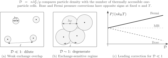
The degeneracy parameter $\mathcal D=n\lambda_T^d/g$ compares particle density with the density of thermally accessible one-particle states. The packet picture is heuristic; the fugacity expansion gives the quantitative criterion. For $\mathcal D\ll1$, Bose and Fermi pressures approach $nk_{\mathrm B}T$ from opposite sides at fixed $n,T$.

The phrases statistical attraction for bosons and statistical repulsion for fermions summarize these signs. They do not mean that an interparticle potential has appeared. Exchange changes state counting and correlations even when the Hamiltonian contains no force between particles.

Exchange Cycles in the Canonical Ensemble

The two-particle partition function makes the origin of the correction explicit. For two identical noninteracting particles,

$$Z_2^{(\eta)} = \frac{1}{2} \left[ q_1(\beta)^2 + \eta q_1(2\beta) \right].$$

The first term is the Maxwell–Boltzmann contribution $q_1^2/2!$. The second is the two-cycle exchange contribution.

For a free gas in $d$ dimensions,

$$q_1(\beta) = g\frac{V}{\lambda_T^d}$$

and

$$q_1(2\beta) = g\frac{V}{2^{d/2}\lambda_T^d}.$$

Their ratio is

$$\frac{q_1(2\beta)}{q_1(\beta)^2} = \frac{\lambda_T^d} {2^{d/2}gV}.$$

For $N$ particles, the number of possible exchanged pairs grows with $N^2$. The correction to an extensive thermodynamic quantity is therefore controlled per particle by

$$\frac{N\lambda_T^d}{gV} = \mathcal D,$$

not by $\lambda_T^d/V$ alone. The recurrence and higher permutation cycles are developed in Partition Functions.

Occupation Fluctuations

An ideal quantum mode has

$$\operatorname{Var}(n_i) = f_\eta(\epsilon_i) \left[ 1+ \eta f_\eta(\epsilon_i) \right].$$

For $f_\eta\ll1$,

$$\operatorname{Var}(n_i) = f_\eta + \eta f_\eta^2 + O(f_\eta^3).$$

The leading Maxwell–Boltzmann result is Poisson-like,

$$\operatorname{Var}(n_i) \simeq \overline n_i.$$

Bosons have a positive bunching correction; fermions have a negative exclusion correction. The distinction survives first in quantities of second order in the small occupation.

The exact probability laws are still different: a bosonic mode is geometric, while a fermionic mode is Bernoulli. They become observationally close only because events with more than one particle in the same dilute mode are already of order $f_i^2$.

Internal Degeneracy and Mixtures

The factor $g$ needs a physical interpretation. If $g$ orthogonal internal states have equal energy, equal chemical potential, and equal populations, then each component has density approximately $n/g$. Exchange operates only between particles in the same orthogonal internal state, giving

$$\mathcal D = \frac{n\lambda_T^d}{g}.$$

For a mixture with component densities $n_a$, the safer criteria are

$$n_a\lambda_{T,a}^d \ll1$$

for every identical component $a$. A single total-$g$ formula can fail when populations are polarized, masses differ, chemical potentials differ, or internal states are not conserved.

If component particle numbers are separately fixed, the Maxwell–Boltzmann canonical factor is

$$Z_{\mathrm{MB}} \simeq \prod_a \frac{q_{1,a}^{N_a}}{N_a!},$$

not one denominator $(\sum_aN_a)!$ for physically distinguishable species.

Internal degeneracy weakens exchange corrections at fixed total density because particles are distributed among more orthogonal one-particle states. It does not make particles of the same internal state distinguishable.

Relation to the Fermi Temperature

For a homogeneous three-dimensional ideal Fermi gas with equal population of $g$ components,

$$n = g\frac{k_{\mathrm F}^3}{6\pi^2}$$

and

$$k_{\mathrm B}T_{\mathrm F} = \frac{\hbar^2k_{\mathrm F}^2}{2m}.$$

The degeneracy parameter becomes

$$\mathcal D = \frac{4}{3\sqrt\pi} \left( \frac{T_{\mathrm F}}{T} \right)^{3/2}.$$

Thus

$$T\gg T_{\mathrm F}$$

is the Fermi-gas form of the Maxwell–Boltzmann criterion. The numerical coefficient depends on the convention used to define $T_{\mathrm F}$ and on dimensionality, but the parametric statement does not.

For an ideal uniform Bose gas, quantum degeneracy becomes important when $n\lambda_T^3/g$ is of order one. Bose–Einstein condensation in three dimensions occurs at

$$\frac{n\lambda_T^3}{g} = \zeta(3/2)$$

under the standard ideal-gas and component assumptions. The Maxwell–Boltzmann regime lies parametrically far from that threshold.

Dimensionality

The general free-particle criterion is

$$\mathcal D_d = \frac{n_d\lambda_T^d}{g} \ll1,$$

where $n_d=N/V_d$ is the $d$-dimensional density. The leading ideal exchange correction is

$$\frac{P}{n_dk_{\mathrm B}T} = 1 - \eta \frac{\mathcal D_d}{2^{1+d/2}} + O(\mathcal D_d^2).$$

Changing dimension changes the density of states, the powers in the fugacity expansion, infrared behavior, and condensation criteria. One must not insert a three-dimensional $n\lambda_T^3$ into a quasi-one-dimensional or quasi-two-dimensional gas without first deciding which transverse levels are thermally active.

If transverse gaps greatly exceed $k_{\mathrm B}T$, the gas is effectively lower dimensional. If many transverse levels are populated, the full trapped or anisotropic one-particle partition function should be used instead of a pure $d$-dimensional continuum formula.

Trapped and Inhomogeneous Gases

For a slowly varying potential $V(\mathbf r)$, the local semiclassical occupation is

$$f_\eta(\mathbf r,\mathbf p) = \frac{1}{ z^{-1} e^{\beta[\mathbf p^2/(2m)+V(\mathbf r)]} - \eta }.$$

Define the local activity

$$y(\mathbf r,\mathbf p) = z e^{-\beta[\mathbf p^2/(2m)+V(\mathbf r)]}.$$

The Maxwell–Boltzmann approximation requires the maximum relevant $y$ to be small. At leading order,

$$n(\mathbf r) \simeq \frac{g}{\lambda_T^d} z e^{-\beta V(\mathbf r)},$$

so the local degeneracy parameter is

$$\mathcal D(\mathbf r) = \frac{n(\mathbf r)\lambda_T^d}{g} \simeq z e^{-\beta V(\mathbf r)}.$$

The center of a trapped cloud can be quantum degenerate while its dilute wings remain Maxwell–Boltzmann. A criterion based only on the cloud-averaged density can miss this coexistence of regimes.

For a high-temperature $d$-dimensional harmonic trap with frequency $\omega$,

$$q_1 \simeq g \left( \frac{k_{\mathrm B}T}{\hbar\omega} \right)^d.$$

A useful global estimate is

$$\frac{N}{q_1} \ll1,$$

but local central occupation remains the sharper diagnostic.

Finite and Discrete Spectra

The continuum thermal wavelength is not universal. In a small box, lattice, molecule, or finite trap, the exact one-particle spectrum may be sparse. The robust criterion is

$$\max_i e^{-\beta(\epsilon_i-\mu)} \ll1.$$

If this holds, the occupation expansion is classical even when the sum over states cannot be replaced by a momentum integral. The one-particle partition function should remain

$$q_1(\beta) = \sum_i e^{-\beta\epsilon_i}$$

rather than being forced into $gV/\lambda_T^d$.

Conversely, a continuum approximation can be excellent while $z$ is not small. A degenerate Fermi gas in a macroscopic box has nearly continuous levels but is not Maxwell–Boltzmann.

On a lattice, low filling can help suppress exchange occupancy effects, but the band width, lattice spacing, multiple orbitals, and interactions replace the simple free-space thermal-wavelength picture. Low fugacity and small mode occupations remain the portable criteria.

Massless and Nonconserved Quanta

For photons and phonons in equilibrium, particle number is not generally conserved and the chemical potential is usually

$$\mu=0.$$

Then

$$y = e^{-\beta\epsilon}.$$

Low-energy modes have $y$ of order one, so the whole equilibrium distribution is not globally Maxwell–Boltzmann. Only the high-energy Wien tail,

$$\beta\epsilon\gg1,$$

has

$$f_{\mathrm B}(\epsilon) \simeq e^{-\beta\epsilon}.$$

Raising the temperature does not create a small fugacity for a species whose equilibrium chemical potential remains zero; it shifts the set of thermally important modes. The homogeneous massive-particle criterion $n\lambda_T^3\ll1$ should not be imported unchanged.

Interactions and the Virial Expansion

Low fugacity also organizes an interacting gas, but the coefficients are no longer determined only by exchange. The density virial expansion has the form

$$\frac{P}{k_{\mathrm B}T} = n + B_2(T)n^2 + B_3(T)n^3 + \cdots.$$

For a one-component ideal quantum gas in three dimensions,

$$B_2^{\mathrm{exchange}} = -\eta \frac{\lambda_T^3}{2^{5/2}}$$

before internal-degeneracy factors are included. With interactions,

$$B_2 = B_2^{\mathrm{exchange}} + B_2^{\mathrm{interaction}}.$$

The interaction contribution can contain scattering phase shifts and bound-state terms. Strong scattering, resonances, or weakly bound molecules can make it important even when exchange degeneracy is modest.

Therefore

$$n\lambda_T^3\ll1$$

does not by itself imply

$$P=nk_{\mathrm B}T.$$

It implies that exchange corrections are small. Ideal-gas behavior additionally requires

$$|B_2(T)|n\ll1,$$

with analogous control of higher virial terms. The Beth–Uhlenbeck relation is the canonical scattering-theory refinement of $B_2^{\mathrm{interaction}}$; its full derivation lies beyond this page.

The ħ → 0 Perspective

At fixed $n$, $T$, and $m$,

$$\lambda_T \propto \hbar,$$

so

$$\hbar\to0$$

drives

$$\mathcal D \to 0.$$

This formal limit suppresses exchange corrections and often supports a phase-space approximation simultaneously. It is only one route to Maxwell–Boltzmann statistics. Holding $\hbar$ fixed and taking $n\to0$ also gives $\mathcal D\to0$, even if one-particle motion retains discrete quantum structure.

Likewise, taking $T\to\infty$ decreases $\lambda_T$ for massive nonrelativistic particles, but an effective Hamiltonian, internal excitation spectrum, ionization threshold, relativistic crossover, or interaction potential may change before the formal limit is reached.

Semiclassical Limits and Correspondence develops the broader action-based classical limit. The present criterion concerns exchange statistics.

Accuracy Estimates

The approximation should be tied to an observable and tolerance.

Mode occupation

For one mode with $y\ll1$,

$$\frac{ f_\eta-y }{y} = \eta y + O(y^2).$$

The relative error is controlled locally by $y$.

Pressure

For a homogeneous free gas,

$$\frac{ P-nk_{\mathrm B}T }{nk_{\mathrm B}T} = -\eta \frac{\mathcal D}{2^{1+d/2}} + O(\mathcal D^2).$$

The numerical coefficient can make the pressure accurate even when $\mathcal D$ is not extremely tiny, but other observables can have larger corrections.

Fluctuation statistics

The relative correction to a one-mode Poisson variance is of order $f_i$. Two-particle coincidences and short-distance correlations are therefore often more sensitive to exchange than the equation of state.

Nonuniform systems

Use the largest local activity or degeneracy parameter in the region sampled by the observable. A global mean can underestimate the error in a dense center.

Terms labeled $O(\mathcal D^2)$ also require the fugacity expansion to be regular. Near a singularity, bound-state threshold, condensation point, or phase transition, a low-order truncation may fail before a naive numerical estimate suggests.

Regime Dictionary

Statement	What it controls	What it does not guarantee
$e^{-\beta(\epsilon_i-\mu)}\ll1$ for relevant modes	Bose/Fermi occupation approaches Boltzmann occupation	continuum phase-space integral
$n\lambda_T^d/g\ll1$	exchange degeneracy in a homogeneous free gas	weak interactions
$\beta\Delta E\ll1$	unresolved discrete level spacing	small fugacity
$\lambda_T/L\ll1$	local semiclassical variation	ideal-gas equation of state
$	B_2	n\ll1$ and higher virial control
$T\gg T_{\mathrm F}$	nondegenerate homogeneous Fermi gas	classical motion in every external potential
$\overline n_i\gg1$ for bosons	possible classical-field regime	Maxwell–Boltzmann statistics

Practical Workflow

1. Identify whether particle number is conserved and whether a chemical potential is meaningful.
2. Set and state the one-particle energy-zero convention.
3. List internal components and decide which particles are mutually identical.
4. Inspect the invariant mode activities $e^{-\beta(\epsilon_i-\mu)}$.
5. For a homogeneous free gas, compute $n\lambda_T^d/g$.
6. For a trap, compute the local central activity or local phase-space density.
7. Check whether the one-particle continuum approximation is valid independently.
8. Estimate the leading exchange correction for the observable of interest.
9. Check interaction virial coefficients, bound states, and resonances.
10. State the requested accuracy and which terms are neglected.
11. Verify that no dimensional, relativistic, or internal-state crossover intervenes.
12. Use the full Bose or Fermi expression when the diagnostic is not parametrically small.

Common Mistakes

• Treating Maxwell–Boltzmann particles as a third species alongside bosons and fermions.
• Dropping $1/N!$ because exchange is small.
• Using $q_1^N$ for one gas of identical particles.
• Saying only “high temperature” without comparing $T$ with density, mass, and level scales.
• Using $z\ll1$ without fixing the energy zero.
• Treating negative chemical potential as sufficient evidence of classicality.
• Applying $n\lambda_T^3$ to a lower-dimensional gas without changing the density units.
• Using total density divided by $g$ when internal populations are unequal.
• Assuming low exchange degeneracy means weak interactions.
• Extending the first virial correction to $\mathcal D\sim1$ as a controlled formula.
• Calling bosonic high-occupation classical-field behavior Maxwell–Boltzmann.
• Assuming a continuum spectrum implies classical statistics.
• Assuming small occupation implies one-particle trajectories are semiclassical.
• Applying a massive-particle fugacity criterion unchanged to photons or phonons.
• Ignoring that a trapped center and wings can lie in different regimes.

Exercises

Thermal wavelength from the momentum integral

Evaluate

$$q_1 = gV \int \frac{d^dp}{(2\pi\hbar)^d} e^{-\beta p^2/(2m)}$$

and identify $\lambda_T$.

Solution

The Gaussian factorizes into $d$ one-dimensional integrals:

$$\int d^dp\, e^{-\beta p^2/(2m)} = \left( \frac{2\pi m}{\beta} \right)^{d/2}.$$

Therefore

$$\begin{aligned} q_1 &= gV \frac{1}{(2\pi\hbar)^d} \left( \frac{2\pi m}{\beta} \right)^{d/2} \\ &= gV \left( \frac{m}{2\pi\beta\hbar^2} \right)^{d/2}. \end{aligned}$$

Defining

$$\lambda_T = \sqrt{ \frac{2\pi\beta\hbar^2}{m} }$$

gives

$$q_1 = g\frac{V}{\lambda_T^d}.$$

Occupation expansion and sign

Starting from

$$f_\eta = \frac{y}{1-\eta y},$$

derive the first three terms for bosons and fermions. What is the relative error of the Maxwell–Boltzmann approximation at leading order?

Solution

For $|y|<1$,

$$\frac{1}{1-\eta y} = 1+\eta y+y^2+O(y^3),$$

because $\eta^2=1$. Hence

$$f_\eta = y+\eta y^2+y^3+O(y^4).$$

For bosons,

$$f_{\mathrm B} = y+y^2+y^3+O(y^4),$$

while for fermions,

$$f_{\mathrm F} = y-y^2+y^3+O(y^4).$$

Since $f_{\mathrm{MB}}=y$,

$$\frac{f_\eta-f_{\mathrm{MB}}} {f_{\mathrm{MB}}} = \eta y+O(y^2).$$

Bosons lie above and fermions below the Boltzmann occupation at the first correction.

Derive the second virial correction

In $d$ dimensions, use

$$\mathcal D = z+ \eta\frac{z^2}{2^{d/2}} +O(z^3)$$

and

$$\frac{P\lambda_T^d}{gk_{\mathrm B}T} = z+ \eta\frac{z^2}{2^{1+d/2}} +O(z^3)$$

to express $P/(nk_{\mathrm B}T)$ in powers of $\mathcal D$.

Solution

Invert the density series:

$$z = \mathcal D - \eta \frac{\mathcal D^2}{2^{d/2}} +O(\mathcal D^3).$$

Substitute into the pressure series and keep second order:

$$\begin{aligned} \frac{P\lambda_T^d}{gk_{\mathrm B}T} = {}&\mathcal D - \eta \frac{\mathcal D^2}{2^{d/2}} \\ &+ \eta \frac{\mathcal D^2}{2^{1+d/2}} + O(\mathcal D^3) \\ = {}&\mathcal D - \eta \frac{\mathcal D^2}{2^{1+d/2}} + O(\mathcal D^3). \end{aligned}$$

Because $n=g\mathcal D/\lambda_T^d$,

$$\frac{P}{nk_{\mathrm B}T} = 1 - \eta \frac{\mathcal D}{2^{1+d/2}} + O(\mathcal D^2).$$

Two-particle exchange term

For a three-dimensional free gas, compare the exchange term with the Maxwell–Boltzmann term in

$$Z_2^{(\eta)} = \frac12 \left[ q_1(\beta)^2 + \eta q_1(2\beta) \right].$$

Assume internal degeneracy $g$.

Solution

In three dimensions,

$$q_1(\beta) = g\frac{V}{\lambda_T^3}$$

and

$$q_1(2\beta) = g\frac{V}{2^{3/2}\lambda_T^3}.$$

The magnitude ratio is

$$\frac{q_1(2\beta)}{q_1(\beta)^2} = \frac{\lambda_T^3} {2^{3/2}gV}.$$

For exactly two particles this vanishes as $V^{-1}$. In an $N$-particle gas the number of candidate pairs grows as $N^2$, so the correction per particle is controlled by $N\lambda_T^3/(gV)=n\lambda_T^3/g$.

Energy-zero invariance

Show that $z\ll1$ is convention dependent but $e^{-\beta(\epsilon_i-\mu)}\ll1$ is not.

Solution

Under

$$\epsilon_i' = \epsilon_i+C, \qquad \mu' = \mu+C,$$

the fugacity becomes

$$z' = e^{\beta\mu'} = e^{\beta C}z.$$

Its numerical size changes. The mode activity is

$$z'e^{-\beta\epsilon_i'} = e^{\beta C}z e^{-\beta(\epsilon_i+C)} = ze^{-\beta\epsilon_i}.$$

Equivalently, $\epsilon_i'-\mu'=\epsilon_i-\mu$. Small mode activity is the invariant condition. One may use $z\ll1$ after setting the lowest one-particle energy to zero.

Unequal internal populations

A two-component gas has equal masses but densities $n_\uparrow$ and $n_\downarrow$. State the classicality criterion and the leading ideal exchange contribution to the pressure in three dimensions.

Solution

The two orthogonal components exchange only within themselves. The criteria are

$$n_\uparrow\lambda_T^3\ll1, \qquad n_\downarrow\lambda_T^3\ll1.$$

For fermionic components, each contributes

$$P_a = n_ak_{\mathrm B}T \left[ 1+ \frac{n_a\lambda_T^3}{2^{5/2}} + O \left( n_a^2\lambda_T^6 \right) \right].$$

Thus

$$\begin{aligned} P = {}& (n_\uparrow+n_\downarrow)k_{\mathrm B}T \\ &+ \frac{k_{\mathrm B}T\lambda_T^3}{2^{5/2}} \left( n_\uparrow^2+n_\downarrow^2 \right) + \cdots. \end{aligned}$$

Only for equal populations can this be rewritten with total density and $g=2$ in the simple form used in the main text.

Classical wings of a trapped gas

In the local-density approximation, let

$$n(\mathbf r) \simeq \frac{g}{\lambda_T^d} z e^{-\beta V(\mathbf r)}.$$

Show why the wings can be Maxwell–Boltzmann even when the center is degenerate.

Solution

The local degeneracy parameter is

$$\mathcal D(\mathbf r) = \frac{n(\mathbf r)\lambda_T^d}{g} \simeq z e^{-\beta V(\mathbf r)}.$$

Choose the potential minimum so that $V(\mathbf0)=0$. The center has

$$\mathcal D(\mathbf0) \simeq z.$$

As $V(\mathbf r)$ grows into the wings,

$$\mathcal D(\mathbf r) = \mathcal D(\mathbf0) e^{-\beta V(\mathbf r)}$$

falls exponentially. The center can have $\mathcal D$ of order one while sufficiently distant regions have $\mathcal D\ll1$. A cloud-averaged density obscures this local distinction.

Fermi temperature criterion

For a homogeneous three-dimensional gas with

$$n = g\frac{k_{\mathrm F}^3}{6\pi^2}, \qquad k_{\mathrm B}T_{\mathrm F} = \frac{\hbar^2k_{\mathrm F}^2}{2m},$$

derive $\mathcal D$ in terms of $T/T_{\mathrm F}$.

Solution

Use

$$\lambda_T^3 = \left( \frac{2\pi\hbar^2}{mk_{\mathrm B}T} \right)^{3/2}.$$

Since

$$\frac{\hbar^2}{mk_{\mathrm B}T} = \frac{2}{k_{\mathrm F}^2} \frac{T_{\mathrm F}}{T},$$

one finds

$$\lambda_T^3 = \frac{(4\pi)^{3/2}}{k_{\mathrm F}^3} \left( \frac{T_{\mathrm F}}{T} \right)^{3/2}.$$

Therefore

$$\begin{aligned} \mathcal D &= \frac{n\lambda_T^3}{g} \\ &= \frac{k_{\mathrm F}^3}{6\pi^2} \frac{(4\pi)^{3/2}}{k_{\mathrm F}^3} \left( \frac{T_{\mathrm F}}{T} \right)^{3/2} \\ &= \frac{4}{3\sqrt\pi} \left( \frac{T_{\mathrm F}}{T} \right)^{3/2}. \end{aligned}$$

Hence $T\gg T_{\mathrm F}$ is equivalent to $\mathcal D\ll1$ up to an order-one coefficient.

Further Deductions

• Maxwell–Boltzmann statistics is an asymptotic regime of both Bose and Fermi systems, not a replacement exchange postulate.
• The thermal wavelength enters because it converts a volume into a count of thermally accessible one-particle phase-space cells.
• The small parameter is component-resolved phase-space density, not temperature alone.
• Fugacity expansions organize exchange cycles: the $z^\ell$ term carries an $\ell$-cycle contribution.
• Bose and Fermi thermodynamics first differ from Boltzmann thermodynamics at second order in fugacity.
• Pressure can look nearly classical while coincidence correlations or occupation fluctuations still reveal exchange more clearly.
• Diluteness suppresses exchange but does not erase interactions, bound states, discrete geometry, or relativistic changes of dispersion.
• A local criterion is required in traps; different parts of one equilibrium cloud can occupy different statistical regimes.

Cross-Links

• Quantum Statistics Overview
• Maxwell–Boltzmann Limit
• Grand-Canonical Ensemble
• Partition Functions
• Chemical Potential
• Bose–Einstein Statistics
• Fermi–Dirac Statistics
• Ideal Bose Gas
• Ideal Fermi Gas
• Identical Particles
• Thermodynamic Limit
• Semiclassical Limits and Correspondence
• Ensemble Formula Sheet

References

1. G. E. Uhlenbeck and L. Gropper, “The Equation of State of a Non-Ideal Einstein–Bose or Fermi–Dirac Gas”, Physical Review 41, 79–90 (1932).
2. E. Beth and G. E. Uhlenbeck, “The Quantum Theory of the Non-Ideal Gas. II. Behaviour at Low Temperatures”, Physica 4, 915–924 (1937).
3. R. K. Pathria and P. D. Beale, Statistical Mechanics, 4th ed., Elsevier (2021), chapters 6–8.
4. K. Huang, Statistical Mechanics, 2nd ed., Wiley (1987), chapters 9–12.
5. M. Kardar, Statistical Physics of Particles, Cambridge University Press (2007), chapters 5–7.
6. L. D. Landau and E. M. Lifshitz, Statistical Physics, Part 1, 3rd ed., Butterworth–Heinemann (1980), sections 40–58.
7. R. Balian, From Microphysics to Macrophysics, Volume I, Springer (1991), chapters 7–9.